CPU-Only Energy Load Forecasting: What a New ERCOT Benchmark Reveals About TSFMs Without GPUs

Most discussions of TSFM inference assume GPU access: batch sizes of hundreds, A10G or A100 cards, throughput measured in thousands of series per second. That is the right framing for a cloud API serving millions of requests. It is the wrong framing for a rural cooperative, a university research group, or a small utility running day-ahead scheduling from a laptop in a grid-operations center.

A benchmark published in February 2026—Time Series Foundation Models for Energy Load Forecasting on Consumer Hardware: A Multi-Dimensional Zero-Shot Benchmark by Luigi Simeone—fills this gap directly. It runs four TSFMs against ERCOT hourly load data entirely on consumer-grade hardware (AMD Ryzen 7 8845HS, 16 GB RAM, no dedicated GPU) and evaluates them across four axes that matter for grid operations: context length sensitivity, probabilistic calibration, robustness under distribution shift, and operational prescriptive value. A companion study published in IEEE Access—Meyer et al., Benchmarking Time Series Foundation Models for Short-Term Household Electricity Load Forecasting—reinforces several of the same findings at the household level with German and UK datasets.

Together, these papers answer a question that the energy sector has been asking since Chronos launched: can zero-shot TSFMs replace fitted baselines in production energy forecasting, on hardware that most organizations actually have?

#The Benchmark Setup

Simeone uses ERCOT system-wide hourly demand from January 2020 through December 2024—43,732 observations, measured in megawatts, spanning three operationally distinct regimes: normal operations (2022–2024), the COVID-19 lockdown period (March–April 2020, a 15–20% demand reduction with shifted diurnal patterns), and Winter Storm Uri (February 2021, a cascading grid failure with demand first spiking from extreme heating load, then collapsing under load shedding). ERCOT serves approximately 90% of Texas's electric load across over 26 million customers, making it one of the most heterogeneous and stress-tested grids in the United States.

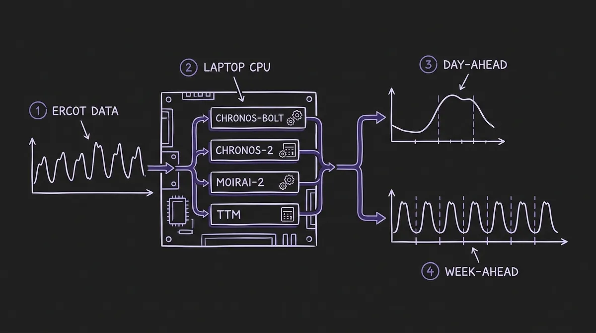
The hardware constraint is deliberate: an AMD Ryzen 7 8845HS with 16 GB system RAM and no GPU. The rationale is explicit in the paper—utilities, cooperatives, and researchers lacking cloud or HPC access need to know whether these models actually run. The benchmark evaluates over 2,352 individual forecast instances across eight context lengths (24 to 2048 hours), two forecast horizons (day-ahead at H=24 and week-ahead at H=168), and three test periods.

The four evaluated TSFMs are:

• Chronos-Bolt (~48M parameters): T5-based encoder-decoder with patch tokenisation, producing 9 direct quantile forecasts rather than autoregressive token rollout. The paper uses the Small variant.
• Chronos-2 (~120M parameters): Encoder-only architecture with group attention for multivariate/covariate inputs, used here in univariate zero-shot mode.
• Moirai-2 (~11M parameters): Decoder-only universal transformer with quantile loss and multi-token prediction, pre-trained on 36 million series (~295 billion observations) including the LOTSA dataset, KernelSynth data, and operational telemetry. The Small variant.
• TinyTimeMixer (TTM) (<1M parameters): MLP-Mixer on patched time series, designed for edge deployment. The r2 variant.

Baselines include Prophet (Facebook's additive decomposition model, widely used in operational energy forecasting), SARIMA, and Seasonal Naive (repeating values from 168 hours prior, the MASE denominator).

#Context Length: Where Foundation Models Win Structurally

The most dramatic finding in the benchmark is the context length sensitivity experiment. The results expose a structural difference between foundation models and fitted baselines that goes beyond accuracy on a single leaderboard row.

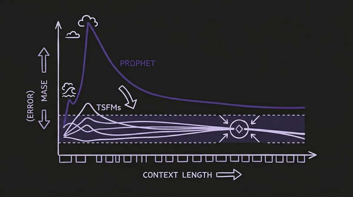
At C=24 hours—one day of history—Prophet produces a mean MASE exceeding 74. That is not a bad forecast; it is a numerical failure. The mechanism is clear: Prophet must estimate weekly Fourier coefficients from a window that is one-seventh of the weekly period. With 24 observations and 25 default trend changepoints, the model has more parameters to estimate than data points to estimate them from. The Stan optimizer produces degenerate coefficients. At C=48 hours, MASE is still above 12; it only drops below 1.0 (Seasonal Naive equivalence) at C=336 hours—two full weekly cycles.

Foundation models behave entirely differently. Chronos-Bolt achieves MASE 0.549 at C=24 hours. Not its best, but operationally usable—sub-1.0, better than repeating last week. The model does not need 24 hours of data to learn that electricity demand follows a diurnal cycle, because it already learned that from millions of series during pre-training. The context window is not a training set; it is a conditioning signal.

By C=512 hours (roughly three weeks of history), the top three foundation models converge tightly: Chronos-Bolt (MASE 0.33), Chronos-2 (0.34), and Moirai-2 (0.33). A Diebold-Mariano test across 720 aligned error values confirms these differences are not statistically significant (p > 0.05 for all pairwise comparisons). TTM sits at 0.43 at C=512, a meaningful gap attributable to its patch-based architecture struggling with very short inputs. At C=24, TTM achieves MASE 5.73—high initial error but not the catastrophic failure of Prophet, and TTM converges to competitive accuracy by C=1024.

The top three foundation models continue improving without saturation as context extends to 2048 hours (Chronos-Bolt 0.315, Moirai-2 0.307 after a 76% relative improvement from its C=24 starting point of 1.304). This suggests that operators with months of historical data could extract further accuracy gains by providing full multi-month context windows—a design choice that is essentially free in CPU inference, since memory rather than GPU compute is the binding constraint.

Meyer et al.'s household-level benchmark at Paderborn University reinforces the context-length finding from a different angle. Across 300+ households from four European datasets (Southern Germany, Lower Saxony, REFIT, IDEAL), they find that TSFMs "outperform all TFS models when the input size increases"—the zero-shot advantage grows with available history. This is the opposite of the conventional wisdom that models trained on task-specific data should dominate on tasks they were trained for.

#Calibration: Where the Models Diverge

Since the top three foundation models are statistically indistinguishable on MASE at C=512, point accuracy cannot drive model selection for energy applications. The benchmark's calibration analysis reveals sharp differences that matter for grid operators who need prediction intervals for reserve planning.

Chronos-2 produces well-calibrated probabilistic forecasts: 95.1% empirical coverage at the 90% nominal level—5.1 percentage points above the target, slightly conservative. For grid operations, this direction of miscalibration is operationally safe: it leads to over-provisioning reserves rather than under-provisioning. During extreme load events (demand exceeding the 95th percentile), Chronos-2 maintains ~100% coverage for extreme highs and ~95% for extreme lows.

Chronos-Bolt is slightly overconfident: 86.1% empirical coverage at the 90% nominal level, meaning roughly 4% more observations fall outside predicted intervals than the model indicates. This is the smallest absolute deviation from the 90% target but in the less-safe direction for reserve planning. Its CRPS (Continuous Ranked Probability Score) of 1,007 MW is the best among all models.

Moirai-2 exhibits problematic overconfidence: ~70% empirical coverage at the 90% nominal level. Roughly 20% of the time, actual demand falls outside what the model considers the plausible range. For reserve procurement, this is operationally dangerous. The authors note that Moirai-2's restricted sampling range (0.05–0.95 probability) during post-hoc quantile interpolation may partially explain the overconfidence.

TTM achieves 100% empirical coverage by producing prediction intervals so wide they contain every observation. Its normalised interval width is 0.32 versus 0.08 for Chronos-Bolt—four times wider than necessary. TTM does not natively produce distributional forecasts in zero-shot mode; uncertainty is approximated by adding Gaussian noise scaled to 10% of the mean forecast magnitude. The result is operationally useless for reserve planning.

The practical implication: if you are building a probabilistic pipeline for conformal or calibrated intervals, Chronos-2 is the default choice for energy applications where safe over-coverage is preferable to under-coverage. If you are optimizing for CRPS and can tolerate a 4-point calibration shortfall, Chronos-Bolt wins on raw probabilistic scoring.

#Robustness Under Distribution Shift

Beyond normal operations, the benchmark tests each model under conditions that have actually broken grid operations. Results at C=512, H=24 relative to a normal summer baseline:

Period	Chronos-Bolt	Chronos-2	Moirai-2	TTM	Prophet
Normal Summer (ref.)	0.342	0.329	0.378	0.456	0.653
COVID Lockdown	0.308 (−10%)	0.290 (−12%)	0.319 (−16%)	0.452 (−1%)	0.657 (+1%)
Winter Storm Uri	0.930 (+172%)	0.879 (+168%)	0.861 (+128%)	1.216 (+167%)	1.498 (+129%)
Holiday Period	1.076 (+215%)	0.864 (+163%)	0.894 (+137%)	1.487 (+226%)	1.224 (+87%)

Under COVID lockdowns, foundation models improved: demand became more predictable as commercial activity regularised, and the models' lower variance captured this. Chronos-2 achieved MASE 0.290 during lockdowns, its best absolute score in the entire study.

Under Winter Storm Uri—a black-swan event that caused grid failure and involuntary load shedding—all models degrade substantially, but Moirai-2 shows the lowest relative degradation (+128% versus +168% for Chronos-Bolt). The benchmark's authors attribute this to Moirai-2's pre-training corpus, which extends LOTSA with KernelSynth synthetic data and operational telemetry from diverse domains including healthcare and finance, giving the model exposure to distributional tails that pure energy-domain training would not cover.

For practitioners building contingency-planning systems that must survive black-swan grid events, Moirai-2's tail robustness may outweigh its calibration deficiencies—but only if post-hoc conformal recalibration is applied to fix the 70% coverage problem.

#Inference on Consumer Hardware

Table 4 from the benchmark measures per-forecast inference time on the AMD Ryzen 7 8845HS:

• TTM: Sub-millisecond. Suitable for real-time edge deployment and sub-second dashboards.
• Chronos-Bolt / Chronos-2: ~31–100 ms per 24-hour forecast at representative context lengths. Adequate for day-ahead operational cycles and near-real-time micro-batch pipelines.
• Prophet: ~700 ms including fitting. Adequate for infrequent batch jobs but a bottleneck if forecasts are needed across thousands of meters.
• SARIMA: ~6.2 seconds at C=2048. Impractical for large-scale CPU deployment.

An important nuance the authors flag: comparing inference-only time for foundation models against fit-plus-inference time for Prophet is methodologically asymmetric. Foundation models amortise their training cost to the model developer—the operational user receives a pre-trained artifact. The speed advantage is real, but partly represents a cost shift from user to developer. For practitioners evaluating total cost of ownership, this is worth accounting for, though for most energy organizations the benefit is unambiguously positive.

TimesFM was excluded from the benchmark because it "requires GPU acceleration for inference within reasonable time." This is a real deployment constraint that the GPU optimization discussion implicitly assumes away.

#Prescriptive Analytics: What the Probabilistic Forecasts Are Worth

The benchmark extends beyond accuracy metrics to quantify operational value. Using Chronos-Bolt's probabilistic forecasts for a representative summer peak period:

Reserve margin optimization: A conventional fixed 10% reserve margin approach maintains 99.9% reliability. A probabilistic approach sizing reserves to the 99.9th percentile of the forecast distribution achieves the same reliability target while reducing average reserve capacity by 63.8%. For a grid the size of ERCOT—peaking at ~75,000 MW—this represents thousands of megawatts of avoided reserve procurement, translating to substantial cost savings in capacity markets.

Peak detection: Using the 95th percentile of the predictive distribution as a threshold, Chronos-Bolt correctly identifies 46% of peak hours with a 12.5% false positive rate. This is sufficient for pre-positioning demand response resources, where the cost of a false alarm is low relative to missing a peak event.

The storage optimization case study is instructive in a different way: it illustrates a period where the price spread between overnight and morning hours is insufficient to cover cycling costs, producing negative net benefit. This is a realistic outcome that a naive point-forecast system might miss. Probabilistic forecasts make the uncertainty explicit, allowing a storage operator to make better-informed decisions about whether to dispatch in a given period.

#Deployment Guidance for Energy Practitioners

Synthesizing both studies, the practical guidance for teams deploying TSFMs on commodity hardware:

If you need day-ahead load forecasts on CPU hardware: Start with Chronos-Bolt (48M parameters, ~31 ms per forecast at C=512). It achieves the best composite score across accuracy, calibration, robustness, and latency. If safe over-coverage is required for reserve planning—as it typically is for grid operators—consider Chronos-2 instead.

If you need robustness to black-swan grid events: Moirai-2 shows the lowest relative degradation under extreme distribution shifts (Winter Storm Uri: +128% vs +168–172% for Chronos models). Apply post-hoc recalibration to address its ~70% coverage problem before using it for reserve planning.

If you are deploying on embedded hardware or IoT gateways: TTM's sub-millisecond CPU inference makes it the only realistic option. Accept that its uncertainty estimates are operationally useless and apply conformal prediction wrappers for calibrated intervals. At C=1024+, TTM achieves MASE competitive with SARIMA.

If you are currently using Prophet: You need C≥336 hours of fitting context before Prophet reaches Seasonal Naive equivalence. Below that, Prophet produces catastrophic failures. Any deployment where context availability is uncertain—new meters, recently connected substations, rolling-window pipelines with configurable history—should use a foundation model instead.

For fine-tuning decisions: Meyer et al. find that domain-specific fine-tuning of TSFMs on household electricity data is a "promising research direction," particularly because zero-shot models approach but don't consistently beat task-specific transformers. If your utility has substantial historical data and can afford fine-tuning runs, the accuracy gap from zero-shot to fine-tuned TTM or Chronos-Bolt may justify the investment.

For routing across model tiers: The model routing decision for CPU-only deployments is simpler than for GPU pipelines. At low-to-medium context (C<168), route everything to Chronos-Bolt or Chronos-2 to avoid TTM's warm-up penalty. At longer context where throughput matters more, TTM's sub-ms inference makes it attractive for high-volume meter portfolios.

#What This Changes

The GPU assumption embedded in most TSFM deployment discussions has obscured a large category of practical use cases. Rural electric cooperatives in the United States serve 42 million people across 56% of the national landmass; the median co-op does not have a GPU cluster. Municipal utilities in Germany, distribution system operators across developing markets, and research groups studying grid edge behavior all share the same constraint.

The Simeone benchmark establishes empirically that four production-ready TSFMs run effectively on commodity hardware for energy load forecasting at forecast horizons and accuracy levels relevant to grid operations. The energy demand case study on this site covered a European utility using TSFM.ai via REST API, which abstracts away the infrastructure question. These new benchmarks answer what happens when you pull the models down and run them locally on a laptop—and the answer, for the right model with sufficient context, is that it works.

The calibration findings are the more practical contribution. Because Chronos-Bolt, Chronos-2, and Moirai-2 are statistically indistinguishable on MASE at operationally relevant context lengths, point accuracy is the wrong selection criterion for energy applications. Calibration, robustness to distribution shift, and inference latency should drive the choice—and on those dimensions, the models differ substantially. For grid applications where over-coverage is preferred over under-coverage in reserve planning, Chronos-2's slightly conservative intervals make it the safer default despite a 5-point deviation from the 90% nominal target.

The streaming inference post on this site noted that TTM's ~95 ms CPU inference makes it viable for near-real-time pipelines. The Simeone benchmark clarifies an important caveat: TTM's uncertainty estimates are synthetic and operationally useless for reserve planning. For energy applications requiring probabilistic outputs, TTM should be treated as a point-forecast model and paired with external calibration.

Test both the Chronos family and Moirai-2 in the TSFM.ai playground before committing to a deployment architecture. If your use case allows GPU access for inference, the GPU optimization guide covers how to scale from the CPU baseline described here to production throughputs.

---

Primary sources: Simeone, Luigi. "Time Series Foundation Models for Energy Load Forecasting on Consumer Hardware: A Multi-Dimensional Zero-Shot Benchmark." arXiv:2602.10848, February 2026. | Meyer, Marcel et al. "Benchmarking Time Series Foundation Models for Short-Term Household Electricity Load Forecasting." IEEE Access, vol. 13, pp. 218141–218153, 2025. | ERCOT hourly demand data sourced via EIA Open Data API.