Encoder-Only, Decoder-Only, and Encoder-Decoder: Architecture Tradeoffs in Time Series Foundation Models

If you understand the basics of how transformers work — attention, self-attention, positional encoding — and you have been evaluating time series foundation models for a forecasting problem, you have probably noticed that model papers describe themselves using one of three architectural labels: encoder-only, decoder-only, or encoder-decoder. These are not cosmetic distinctions. The architectural choice determines how the model processes history, how it generates forecasts, and what practical tradeoffs you inherit when you deploy it.

This post breaks down the three architecture families as they apply to TSFMs, with a bonus section on non-transformer alternatives. The goal is not a paper survey — it is a practical guide to understanding which architecture fits which problem.

A Quick Refresher: What Encoder and Decoder Actually Mean

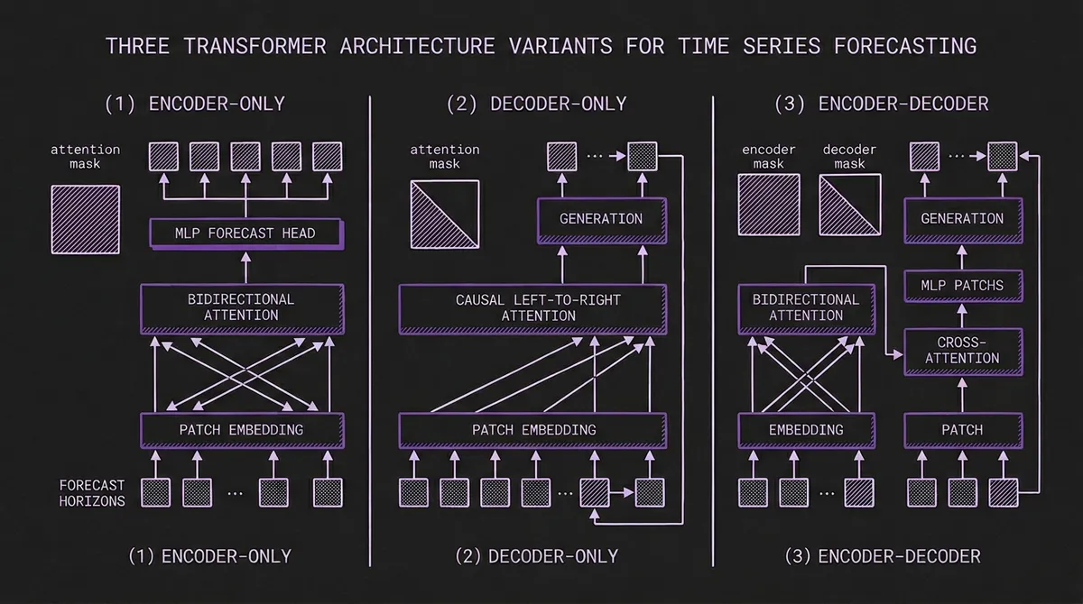
In the original transformer (Vaswani et al., 2017), the encoder reads an input sequence and builds a rich, bidirectional representation of it. Every token attends to every other token, so the encoder can capture relationships across the entire input. The decoder then generates an output sequence one token at a time, attending both to its own previously generated tokens (causal self-attention) and to the encoder's output (cross-attention).

The key distinction is the attention mask:

• Encoder: Bidirectional. Every position sees every other position. The model has full context of the input.
• Decoder: Causal (left-to-right). Each position can only see positions before it. Generation is sequential.
• Encoder-decoder: The encoder is bidirectional over the input; the decoder is causal over the output but also cross-attends to the full encoder representation.

In NLP, encoder-only models (BERT) excel at understanding tasks. Decoder-only models (GPT) excel at generation. Encoder-decoder models (T5) do both. The same intuitions carry over to time series, but with some important twists.

Encoder-Only TSFMs

Key models: Chronos-Bolt (Amazon), MOMENT (CMU), Moirai (Salesforce)

Encoder-only TSFMs process the full historical context through bidirectional self-attention, then produce the entire forecast in a single forward pass through a lightweight output head (typically an MLP or mixture distribution head). There is no autoregressive loop — all forecast steps are generated simultaneously.

How It Works

The input time series is segmented into patches (contiguous subsequences of, say, 32 time steps each). Each patch is linearly projected into the model's hidden dimension, producing a sequence of patch embeddings. The transformer encoder processes these embeddings with full bidirectional attention: every patch can attend to every other patch. The output representation is then mapped to forecast values through a task-specific head.

Because the encoder sees the entire history at once, it can build representations that capture long-range dependencies without the information bottleneck of causal masking. A seasonal pattern at position 10 and its repetition at position 500 are equally accessible during the attention computation.

Why This Architecture Is Fast

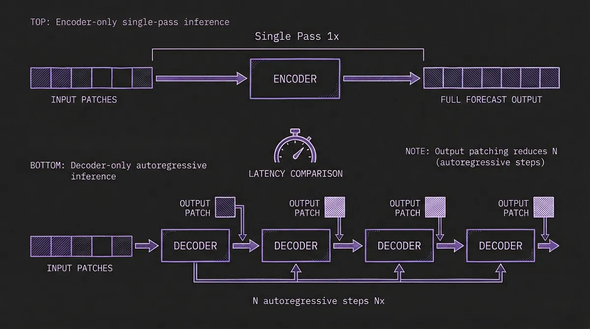
The speed advantage is dramatic. The original Chronos used a T5 encoder-decoder, which required one decoder forward pass per forecast step per sample path. For a 64-step horizon with 20 sample paths, that meant 1,280 decoder passes. Chronos-Bolt dropped the decoder entirely and produces the same forecast in a single forward pass — roughly 250x faster on identical hardware.

Moirai takes a similar approach with its masked encoder and Any-Variate Attention mechanism. The encoder processes all variates and time patches simultaneously, and the mixture distribution head outputs probabilistic forecasts for all steps at once.

Tradeoffs

Strengths:

• Fastest inference — single forward pass, no sequential generation
• Bidirectional attention captures full context without information loss
• Natural fit for multi-task heads (forecasting, anomaly detection, classification, imputation)

Weaknesses:

• Fixed output horizon — the MLP head is typically trained for specific forecast lengths. Producing a different horizon may require a different head or interpolation.
• No "streaming" generation — you cannot generate one step at a time and decide whether to continue. You commit to the full horizon upfront.
• The output head adds an architectural assumption about horizon length that decoder-based models avoid.

When to Choose Encoder-Only

Encoder-only architectures dominate when inference latency matters more than horizon flexibility. If you are forecasting millions of series nightly in a batch pipeline, deploying at the edge on CPU, or serving real-time dashboards, the single-pass property is hard to beat. They also shine when you need multi-task capability — MOMENT's encoder backbone handles forecasting, classification, anomaly detection, and imputation through interchangeable task heads.

Decoder-Only TSFMs

Key models: TimesFM (Google), Toto (Datadog), Lag-Llama, Time-MoE (Alibaba)

Decoder-only TSFMs follow the GPT lineage: they process input causally and generate forecasts autoregressively, one step (or one patch) at a time.

How It Works

The input time series is tokenized — through patching (TimesFM, Toto), lag features (Lag-Llama), or other strategies — and fed to a transformer with causal attention masking. Each position can only attend to positions before it in the sequence. At inference time, the model predicts the next token (or patch), appends it to the sequence, and repeats until the desired horizon is reached.

TimesFM introduced an important optimization: output patching. Instead of predicting a single future value per decoding step, the model produces a patch of multiple future values. With a patch size of 32, a 128-step forecast only requires 4 autoregressive steps instead of 128. This substantially reduces the latency gap with encoder-only models, though it does not eliminate it entirely.

The Scaling Connection

Decoder-only architectures have a major advantage borrowed from the LLM world: they scale predictably. The language modeling community has invested billions of dollars proving that decoder-only transformers improve reliably with more data, more parameters, and more compute. The scaling laws that make GPT-4 and Claude possible apply to decoder-only TSFMs as well.

This is not theoretical. Time-MoE from Alibaba scales to 2.4 billion total parameters using sparse mixture-of-experts (activating only 200M per forward pass), and the accuracy gains follow the expected scaling curves. Timer-S1 from Tsinghua pushes to 8.3 billion parameters with the same architectural family. If the TSFM field follows the trajectory of LLMs — and there are good reasons to think it will — decoder-only is the architecture that benefits most from scale.

Tradeoffs

Strengths:

• Flexible horizons — generate as many or as few steps as needed without retraining
• Proven scaling behavior — more parameters and data reliably improve accuracy
• Natural fit for probabilistic forecasting through sampling (run multiple forward passes, collect trajectory samples)
• Can condition on partial forecasts — useful for scenario analysis and conditional generation

Weaknesses:

• Slower inference due to sequential generation (mitigated but not eliminated by output patching)
• Causal attention means the model cannot "look ahead" — it builds representations strictly left-to-right, which is suboptimal when the full history is available
• Error accumulation — mistakes in early forecast steps propagate through the autoregressive chain
• Generally higher latency per series than encoder-only alternatives

When to Choose Decoder-Only

Decoder-only wins when horizon flexibility and scaling matter more than per-series latency. If you need to forecast varying horizons from a single model, if you are investing in scaling up model size for accuracy, or if you need trajectory-based probabilistic forecasts with full sample paths, decoder-only is the natural choice. It is also the architecture of choice for domain-specific pretraining at scale — Toto's training on 2.36 trillion observability data points follows the decoder-only playbook directly.

Encoder-Decoder TSFMs

Key models: Chronos v1 (Amazon, T5-based), TiDE (Google), classical Temporal Fusion Transformer

Encoder-decoder is the original transformer architecture, and it is the natural fit for sequence-to-sequence problems: the encoder reads input (history), the decoder writes output (forecast). It gives you the best of both worlds — bidirectional understanding of history plus flexible autoregressive generation of forecasts.

How It Works

The encoder processes the historical context with full bidirectional attention, building a rich representation of temporal patterns, trends, and anomalies in the input. The decoder then generates the forecast one step at a time, using causal self-attention over its own previous outputs and cross-attention to the encoder's representation. This cross-attention is the key differentiator: at each generation step, the decoder can selectively attend to any part of the encoded history.

The original Chronos demonstrated this elegantly. It used a T5 (Text-to-Text Transfer Transformer) backbone, mapping binned time series values into a discrete vocabulary. The encoder processed the historical context, and the decoder autoregressively generated forecast tokens, each conditioned on the full encoder representation through cross-attention.

Why the Field Moved Away

If encoder-decoder gives you the best of both worlds, why did the field largely move away from it? The answer is pragmatic: the decoder half is expensive, and the cross-attention is often unnecessary.

In NLP, encoder-decoder models like T5 excel because the input and output are fundamentally different modalities (e.g., English to French, question to answer). The cross-attention bridges this gap. But in time series forecasting, the input and output are the same modality — continuous values over time. The statistical properties of the history are the same as the statistical properties of the forecast. This weakens the case for a separate encoder and decoder with an explicit cross-attention bridge.

Amazon demonstrated this empirically with the Chronos v1 → Chronos-Bolt transition. By removing the decoder and replacing it with a simple MLP head, they achieved:

• 250x faster inference (single pass vs. 1,280 decoder passes for probabilistic forecasts)
• 7% better accuracy on zero-shot benchmarks
• Lower parameter counts at equivalent accuracy (48M Bolt-Small matches 710M Chronos-Large)

The encoder alone was sufficient to capture the temporal patterns, and the MLP head was sufficient to project them into forecast space. The decoder and its cross-attention added compute cost without proportional accuracy benefit.

When Encoder-Decoder Still Makes Sense

Encoder-decoder has not disappeared entirely, and there are scenarios where it remains the right choice:

• Covariate-heavy forecasting: When future known covariates (holidays, promotions, weather forecasts) need to be fed into the decoder alongside the forecast generation, the encoder-decoder split maps cleanly: encoder processes history, decoder processes future covariates plus forecast tokens. Models like TiRex and the Temporal Fusion Transformer use this pattern.
• Heterogeneous input/output: If the input representation (e.g., multivariate sensor data) is structurally different from the output (e.g., a single aggregated forecast), the explicit encoder-decoder bridge can help.
• Tasks beyond forecasting: For sequence-to-sequence tasks like time series translation or temporal summarization, the encoder-decoder structure is more natural than either pure encoder or pure decoder.

Tradeoffs

Strengths:

• Rich bidirectional encoding of history with flexible autoregressive generation
• Natural architecture for covariate-aware forecasting
• Cross-attention allows the decoder to selectively focus on relevant parts of history at each step

Weaknesses:

• Highest computational cost — full encoder pass plus sequential decoder passes plus cross-attention
• The architectural complexity is often unnecessary when input and output share the same modality
• Fewer recent models to choose from as the field has shifted toward simpler architectures

Bonus: Non-Transformer Architectures

Key model: Granite TTM (IBM)

Not every TSFM uses a transformer at all. IBM's Granite TinyTimeMixer replaces self-attention entirely with MLP-Mixer layers, which alternate between mixing information across time positions and across feature channels using simple fully-connected layers.

The result: ~1 million parameters and sub-100ms inference on CPU. No attention mechanism, no autoregressive generation, no GPU required. The model processes patched time series through token-mixing and channel-mixing MLPs, then outputs the full forecast in a single pass.

The accuracy tradeoff is real — Granite TTM matches PatchTST (a 40M-parameter transformer) on short-horizon benchmarks but falls behind on long horizons and complex multivariate settings. But for edge deployment, serverless functions, or scenarios where you need to forecast millions of series at minimal cost, the two-orders-of-magnitude size advantage is decisive.

Comparison Table

	Encoder-Only	Decoder-Only	Encoder-Decoder	Non-Transformer
Attention	Bidirectional	Causal (left-to-right)	Bidirectional encoder + causal decoder	None (MLP mixing)
Generation	Single pass (parallel)	Autoregressive (sequential)	Autoregressive with cross-attention	Single pass (parallel)
Inference Speed	Fast	Moderate (patch output helps)	Slowest	Fastest
Horizon Flexibility	Fixed per head	Fully flexible	Fully flexible	Fixed per head
Scaling Behavior	Good	Best proven	Good	Limited data
Probabilistic Output	Via distribution head	Via sampling trajectories	Via sampling trajectories	Via distribution head
Parameter Efficiency	High	Moderate	Lowest (encoder + decoder + cross-attn)	Highest
Representative Models	Chronos-Bolt, MOMENT, Moirai	TimesFM, Toto, Lag-Llama, Time-MoE	Chronos v1 (T5), TFT	Granite TTM

How to Choose

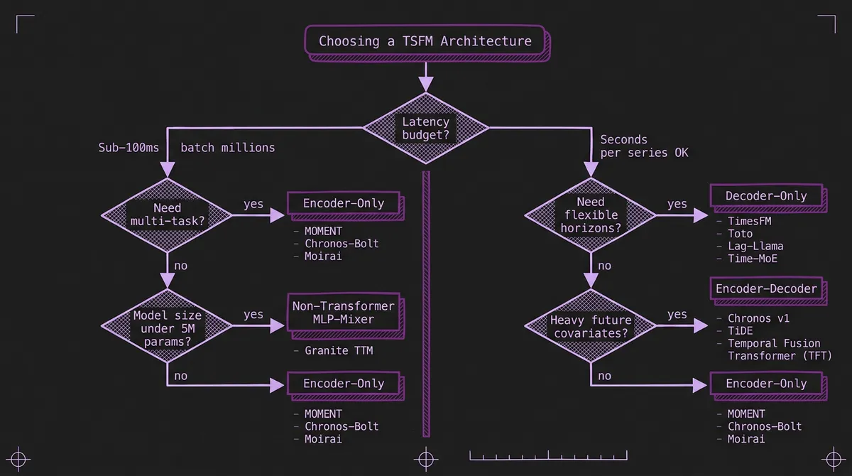
The decision often comes down to three questions:

1. What is your latency budget? If you need sub-100ms per series or are forecasting millions of series in batch: encoder-only or non-transformer. If you have seconds per series and need maximum accuracy: decoder-only at scale.

2. Do you need flexible horizons? If your application requires varying forecast horizons from a single model (e.g., an API that accepts arbitrary horizon requests): decoder-only. If you always forecast the same horizon: encoder-only is simpler and faster.

3. Are you scaling up or scaling down? If your strategy is to throw more data and parameters at the problem for marginal accuracy gains: decoder-only has the most proven scaling curve. If you are optimizing for efficiency, edge deployment, or multi-task versatility: encoder-only or non-transformer.

For most production forecasting workloads in 2026, encoder-only is the pragmatic default. It delivers the best latency-to-accuracy ratio, and the fixed-horizon constraint is rarely an issue since most pipelines forecast at a single cadence. If you need maximum flexibility or are building a general-purpose forecasting platform, decoder-only models give you that at the cost of higher inference compute. Encoder-decoder is increasingly a legacy choice unless you have a specific covariate-heavy architecture that benefits from the explicit cross-attention bridge.

The real answer, of course, is that you do not have to choose just one. TSFM.ai's model routing lets you use the right architecture for each workload — Chronos-Bolt for your batch pipeline, TimesFM for your flexible-horizon API, Granite TTM for your edge sensors — behind a single API.