Timer-S1: Billion-Scale Time Series Forecasting with Serial Scaling

Tsinghua University's Timer model family has grown steadily since 2024, with each generation attacking a different bottleneck in time series foundation models. The original Timer (ICML 2024) established the single-series sequence format and decoder-only pretraining. Timer-XL (ICLR 2025) introduced long-context multi-dimensional attention. Sundial (ICML 2025 Oral) brought flow-matching diffusion and generative probabilistic forecasting. Now, Timer-S1 (Liu, Su, Wang et al., March 2026) targets the scalability bottleneck head-on: how to push a time series model past the billion-parameter mark and actually improve forecasting, not just increase model size.

The result is a sparse Mixture-of-Experts model with 8.3 billion total parameters, 0.75 billion activated per token, and a context length of 11,520 time steps. Evaluated on the GIFT-Eval leaderboard — one of the most comprehensive TSFM benchmarks — Timer-S1 achieves the best MASE (0.693) and CRPS (0.485) scores among pre-trained models. The authors are from Tsinghua University and ByteDance, led by corresponding author Mingsheng Long.

Why Scaling Has Been Hard for TSFMs

There is a well-documented "scaling bottleneck" in time series foundation models. In natural language, scaling to billions of parameters with standard next-token prediction reliably improves capability. In time series, prior attempts to apply the same pattern — larger transformers with mixture-of-experts or simply more layers — have yielded diminishing returns or even inferior performance.

The Timer-S1 authors argue the root cause is a mismatch between training objectives and the nature of forecasting. Time series forecasting is inherently serial: each future value depends on all preceding estimates, and uncertainty compounds step by step. Current approaches sit on two ends of a spectrum:

Parallel forecasting models like Moirai predict multiple future steps simultaneously in a single forward pass. This is fast, but the model never explicitly reasons about dependencies between successive forecast steps. It allocates the same amount of computation to the first predicted step and the hundredth, even though the hundredth carries far more accumulated uncertainty.

Autoregressive next-token prediction (NTP) — used by Chronos, TimesFM, and the original Timer — mirrors the serial nature of the task perfectly. Each step is predicted conditioned on all previous steps. But iterative rolling inference is expensive: to produce a 272-step forecast with patch size 16, the model must roll 17 times, passing through the entire backbone each time. Worse, each step's error feeds into the next, causing error accumulation that is far more severe for time series than for text, because time series lack the self-correcting structure of language.

Timer-S1 introduces a third paradigm — Serial Token Prediction (STP) — that introduces serial computations for long-horizon accuracy while producing multi-step predictions in a single forward pass.

Architecture: TimeMoE Blocks and TimeSTP Blocks

Timer-S1 is a decoder-only transformer composed of three components: a normalization and embedding layer, a transformer backbone built from two types of blocks, and a shared forecasting head.

Normalization and Patch Embedding

Input time series are first instance-normalized: each univariate series is zero-meaned and divided by its standard deviation. This per-instance re-normalization eliminates scale discrepancies between domains and lets the model focus on temporal patterns rather than absolute magnitudes. The same mean and standard deviation are used to de-normalize outputs.

The normalized series is then split into non-overlapping patches of length P = 16, each projected into the model's hidden dimension (D = 1024) via a residual network. A binary mask handles padding for non-divisible lengths. This patch tokenization strategy is shared across the entire model, including both the embedding and output projection layers, ensuring consistent transformation and parameter efficiency.

TimeMoE Blocks (Main Backbone)

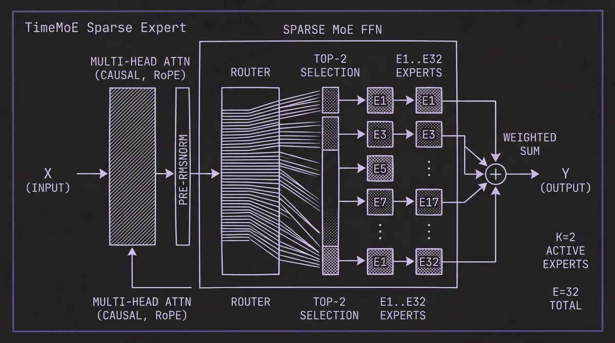
The first L = 24 blocks are sparse MoE transformer layers, each containing multi-head causal self-attention followed by an MoE feed-forward module. The attention uses Rotary Position Embeddings (RoPE) for relative position encoding, along with two stability techniques for billion-scale training: Pre-RMSNorm (normalizing before attention rather than after) and QK-Norm (ℓ₂-normalizing query and key vectors to prevent softmax saturation).

The MoE module in each block contains E = 32 expert feed-forward networks, of which only K = 2 are activated per token via a learned router. The router computes token-to-expert affinity scores and selects the top-2 experts, whose outputs are combined by a weighted sum. An auxiliary load-balancing loss prevents expert collapse — the same mechanism described in our deep dive on Time-MoE, Alibaba's MoE model, though Timer-S1 operates at roughly 3.5× the total parameter scale (8.3B vs 2.4B).

The sparse configuration means 8.3 billion total parameters with only 0.75 billion activated per token. The authors note this aligns with a key property of time series data: global heterogeneity (data from radically different domains) but local simplicity (each patch within a series has relatively straightforward patterns). The MoE structure lets the model store specialized knowledge for many domains without activating all of it for any single input.

TimeSTP Blocks (Serial Forecasting)

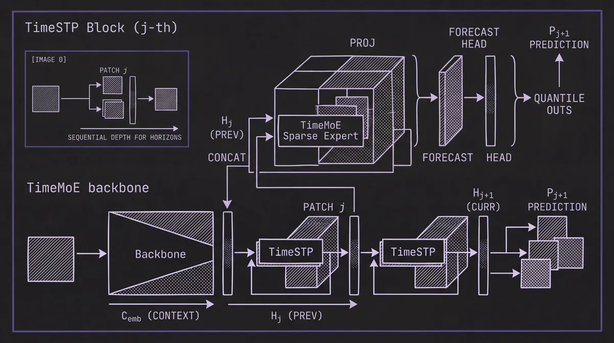
After the 24 main TimeMoE blocks, Timer-S1 appends H = 16 TimeSTP blocks — and this is the architectural innovation. Each TimeSTP block takes the output embeddings from the preceding block, concatenates them with the original input embeddings (from the patch embedding layer), projects the concatenation, and passes the result through its own internal TimeMoE block.

The critical insight is that each TimeSTP block is responsible for predicting the patch that is one step further into the future than the previous block. The j-th TimeSTP block generates predictions shifted by j+1 patches from the input. Because each subsequent block re-attends to the initial context and refines the representation from the previous block, longer-horizon predictions naturally undergo more serial computation — deeper processing for harder predictions.

During inference, all TimeSTP blocks are retained (unlike the similar multi-token prediction used in DeepSeek-V2, which discards auxiliary heads after training). This means Timer-S1 produces a 272-step forecast (17 patches × 16 steps per patch) in a single forward pass. The main blocks process the context once, and each TimeSTP block adds one additional patch prediction. Only the last-token embedding from each level is needed, so inference is efficient: producing the next prediction requires passing through a single TimeSTP block, not the entire backbone.

Forecasting Head

All output embeddings — from both the main blocks and each TimeSTP block — are projected by a shared quantile forecasting head. This head outputs Q = 9 quantile predictions at levels {0.1, 0.2, ..., 0.9}, trained with a weighted quantile loss (an approximation of CRPS). This gives Timer-S1 native probabilistic forecasting capability. The architecture is general enough to swap in alternative heads (linear projection, parametric distributions, or diffusion-based decoders), but the quantile head aligns with the GIFT-Eval evaluation protocol.

Serial Token Prediction vs. NTP vs. MTP

The paper includes direct comparisons between three training objectives using the same backbone configuration:

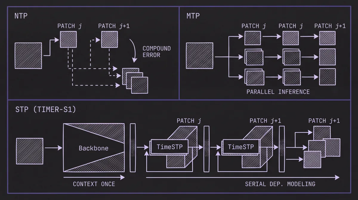
Next-Token Prediction (NTP): Each block predicts the next patch, and inference requires rolling over the entire backbone for each step. At a context length of 11,520, a full forward pass through 40 TimeMoE blocks is needed per roll. For a 272-step forecast, that means 17 full passes.

Multi-Token Prediction (MTP): The backbone predicts multiple patches simultaneously via a larger output head, reducing or eliminating rolling. But the model allocates the same computation to all horizons, missing the serial dependencies that make long-term forecasting hard.

Serial-Token Prediction (STP): Timer-S1's approach. 24 main blocks process the context once, then 16 TimeSTP blocks produce progressively further predictions, each building on the previous. One forward pass produces 17 patches (272 steps).

The results are clear: Timer-S1 with 24 MoE + 16 STP blocks outperforms both Timer-NTP with 40 MoE blocks and Timer-MTP with 40 MoE blocks, using the same total block budget. STP delivers its biggest advantages on medium and long horizons, exactly where serial dependency modeling matters most. Inference time is also lower than NTP because rolling is eliminated, and lower than MTP because the forecasting head is smaller (one patch at a time rather than all at once).

TimeBench: A Trillion-Scale Corpus

Timer-S1 is pre-trained on TimeBench, a curated corpus of over one trillion (10¹²) time points — roughly three times the scale of Time-MoE's Time-300B corpus and an order of magnitude beyond Chronos or Moirai. TimeBench builds on the team's UTSD dataset and incorporates both real-world and synthetic data:

Real-world data is drawn from finance, IoT, meteorology, healthcare, and publicly released corpora from Chronos and Salesforce's LOTSA. Variates are selected using a proxy criterion: statistical significance of fitted ARIMA models, favoring series with strong autoregressive properties.

Synthetic data includes canonical signals (linear, sinusoidal, exponential, impulse, step functions and their combinations) plus KernelSynth-generated series from random-instantiated temporal causal models.

Data quality is ensured through causal mean imputation, outlier removal with k-σ and IQR thresholds using a sliding window, and removal of any instances that could cause test data leakage on GIFT-Eval. Each dataset is profiled on a two-dimensional "complexity plane" using the Augmented Dickey-Fuller test statistic (stationarity) and a forecastability measure based on spectral entropy.

Data Augmentation Against Predictive Bias

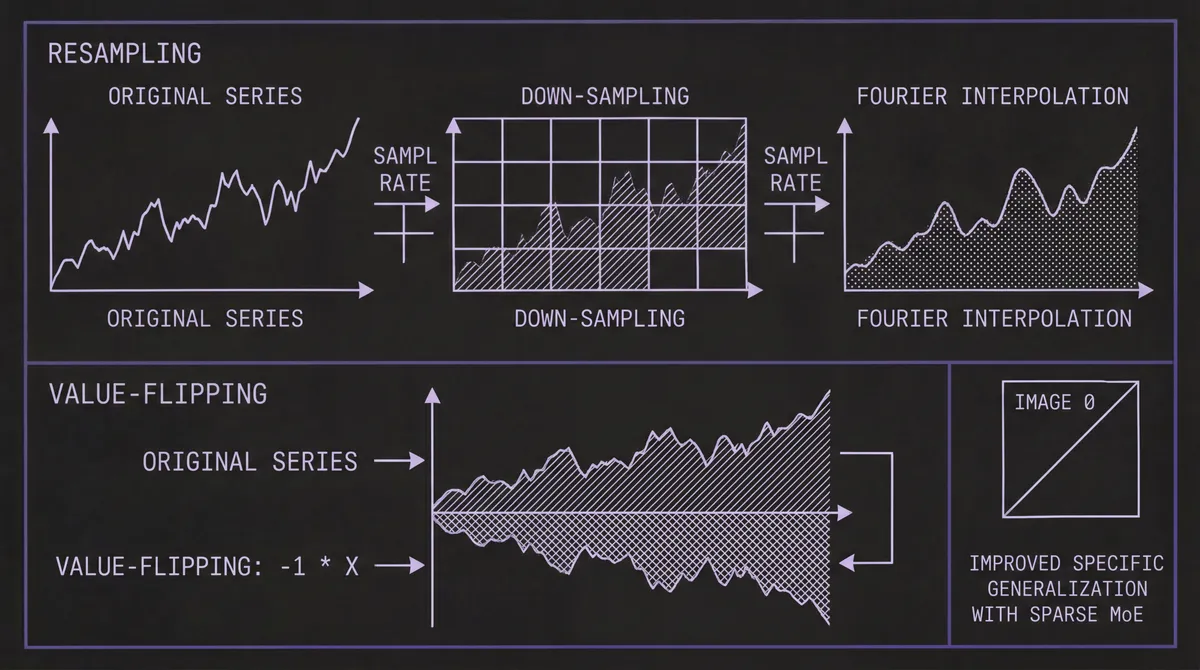
Real-world time series follow imbalanced distributions, which can produce stereotypical tendencies in the trained model. Timer-S1 applies two targeted augmentation techniques:

• Resampling: Varying the sampling rate through down-sampling and Fourier-based interpolation exposes the model to diverse temporal resolutions, improving robustness to frequency shifts.

• Value-flipping: Multiplying both input and output by –1 inverts trends while preserving temporal dependencies. This counteracts the model's tendency to latch onto persistent directional trends — a bias the team explicitly identified in their earlier Sundial work.

The raw data in TimeBench is stored as compressed Parquet files (approximately 4 TB), with an in-memory sliding-window sampler and a hybrid memory-disk loading strategy using 50 MB shards for I/O efficiency.

Post-Training: A Multi-Stage Pipeline

Timer-S1 adapts the pre-training → post-training paradigm from large language models to time series, with three distinct stages:

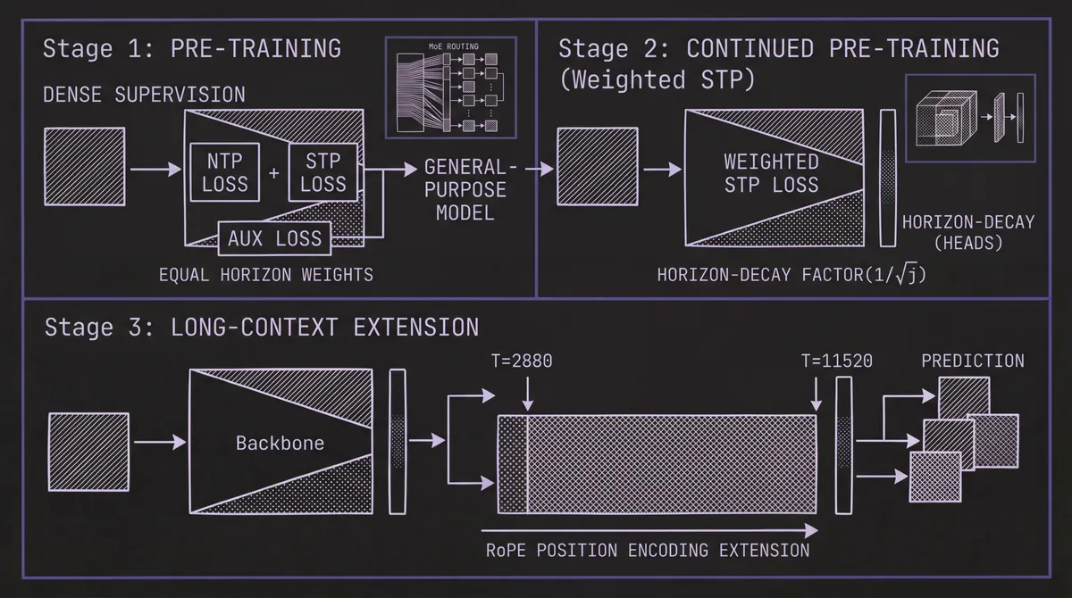
Stage 1: Pre-Training

The model is trained on the full TimeBench corpus with the combined objective: NTP loss + STP loss + auxiliary MoE load-balancing loss, with equal weights across all horizons. Dense supervision is applied — each training sample generates multiple forecasting tasks with variable input and output lengths, maximizing sample efficiency. This stage produces a general-purpose model with uniform performance across horizons. Initial context length is T = 2,880 (180 patches × 16).

Stage 2: Continued Pre-Training (Weighted STP)

Recognizing that long-term accuracy depends fundamentally on short-term precision — the first prediction anchors everything that follows — the post-training stage shifts focus to near-horizon performance. The STP loss is reweighted with a horizon-decay factor of 1/√j for the j-th TimeSTP block. This decay rate is derived from the linear growth of variance in a first-order Markov process: earlier blocks get higher weight, prioritizing short-term accuracy.

Training data at this stage mixes GIFT-Eval pre-training data (focused on short-term tasks) with samples revisited from TimeBench. This data revisiting mechanism prevents overfitting to the narrower post-training distribution while enhancing generalization.

Stage 3: Long-Context Extension

Using the RoPE position encoding, the context window is extended from 2,880 to 11,520 time steps (720 patches). This allows the model to ingest substantially longer histories when available — valuable for series with long-range seasonal or cyclical patterns. For more on why context length matters in time series forecasting, see our dedicated post.

The training infrastructure uses VeOmni, a unified framework for pre-training and post-training at scale, with BF16 precision throughout.

GIFT-Eval Results

The GIFT-Eval benchmark comprises 24 datasets spanning 144,000 time series and 177 million data points across multiple domains. It evaluates both point forecasting (MASE) and probabilistic forecasting (CRPS).

Metric	Timer-S1	Sundial	Improvement
MASE	0.693	0.750	7.6% lower (better)
CRPS	0.485	0.559	13.2% lower (better)

Both scores are the best among pre-trained models on the leaderboard. The improvement over Sundial is especially informative because both models come from the same research group and share the TimeBench training data — the gains are attributable to the MoE architecture, STP objective, and post-training pipeline.

Breaking results down by forecast horizon reveals where the gains come from: Timer-S1 achieves substantially better performance on medium-term and long-term tasks, reinforcing the claim that serial computations in TimeSTP blocks are the key driver. On short-term tasks, the weighted STP post-training keeps Timer-S1 competitive with models explicitly optimized for near-horizon accuracy.

The post-training stages each contribute measurably. Compared to the pre-trained base model, continued pre-training improves performance, and long-context extension adds further gains — validating the multi-stage training approach that has become standard in LLMs.

Scaling Analysis

The paper includes a detailed model configuration study. With TimeSTP fixed at 16 blocks, performance continues to improve as TimeMoE blocks increase up to 24 (the final configuration). With TimeMoE fixed at 24, performance improves as TimeSTP blocks increase up to 16. This confirms the scaling law holds at the billion-parameter level for time series models — a result that was uncertain before this work.

How Timer-S1 Compares

Model	Total Params	Active Params	Architecture	Probabilistic	Context Length
Timer-S1	8.3B	0.75B	Decoder-only MoE + STP	Yes (quantile)	11,520
Time-MoE	2.4B	0.2B	Decoder-only MoE	No	4,096
Sundial	128M	128M (dense)	Flow-matching diffusion	Yes (sampling)	2,880
Chronos-Large	710M	710M (dense)	Encoder-decoder (T5)	Yes (sampling)	512
TimesFM	200M	200M (dense)	Decoder-only	No	2,048
Moirai-Large	311M	311M (dense)	Masked encoder	Yes (mixture)	5,000

Timer-S1 is the first TSFM to cross the billion-parameter scale for activated computations while maintaining efficient inference through sparse MoE routing. Its 11,520 context window is the longest among current TSFMs. For an overview of how different models suit different use cases, see the 2026 TSFM Toolkit guide.

Limitations

The authors are explicit about Timer-S1's constraints:

• No native covariates: Timer-S1 uses the single-series sequence format and does not incorporate exogenous covariates. The team acknowledges this as the largest gap and plans to address it with synthetic multivariate data and an upgraded pre-training framework. For multivariate approaches, see our post on the state of multivariate forecasting.

• Patch size sensitivity: The ablation studies reveal an error spike on sinusoidal signals with a period of approximately 16 — exactly the fixed patch size. This aliasing-like effect is an inherent limitation of patching-based tokenization.

• Inference cost: Although MoE keeps the active parameter count at 0.75B, this is still a larger inference footprint than most alternatives. For latency-sensitive applications, smaller models may be more appropriate. See our post on GPU optimization for TSFM inference.

• Model availability: Timer-S1 weights have not been released at the time of writing. The team's existing models — timer-base-84m and sundial-base-128m — are available on Hugging Face. We will update this post and the model catalog when Timer-S1 weights become available.

What Timer-S1 Means for the Field

Timer-S1 answers a question that has lingered over the TSFM landscape: can time series models benefit from the same scaling strategies that have driven progress in LLMs? The answer appears to be yes — but only with training objectives that respect the serial nature of forecasting. Naive scaling with standard NTP or MTP hits a bottleneck. Serial Token Prediction, by introducing adaptive serial computations across the transformer stack, provides the missing ingredient that unlocks continued scaling.

For practitioners evaluating zero-shot forecasting options, Timer-S1 sets a new performance bar on GIFT-Eval. The combination of MoE efficiency, STP architecture, and a multi-stage training pipeline points toward a maturing recipe for large-scale time series models. Whether fine-tuned or used zero-shot, Timer-S1's approach — serial scaling across architecture, data, and training — will likely influence the next generation of TSFMs.

You can explore the Timer family and other models through the TSFM.ai model catalog and playground, and follow updates on Timer-S1's release on the team's GitHub repository and Hugging Face collection.