Traditional Forecasting vs. TSFMs: The True Cost of Building and Maintaining Enterprise Forecast Pipelines

Every enterprise eventually needs forecasts. Revenue projections for the board. Demand estimates for the supply chain. Capacity plans for infrastructure. The question is never whether to forecast — it is how.

For most organizations, the answer has been the same for decades: assemble a team, choose a methodology, build a pipeline, and maintain it indefinitely. This approach works. It has produced genuine business value across industries. But it carries costs that are rarely quantified upfront and almost always exceed expectations.

Time series foundation models offer a fundamentally different path. Rather than building bespoke forecasting infrastructure, you make an API call. The trade-offs are real, but they are not what most people assume.

This post walks through the full lifecycle of both approaches — honestly, without pretending that either one is universally superior. The numbers may surprise you: industry data shows that 87% of ML models never reach production, full-scale forecasting implementations average 8.7 months to deployment, and McKinsey estimates that only 15% of enterprise ML projects succeed. For forecasting specifically, the odds are worse because the problem compounds data engineering, model development, and domain expertise challenges simultaneously.

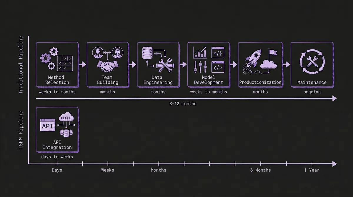
Phase 1: Choosing a Method (Weeks to Months)

Traditional forecasting begins with a decision that most organizations underestimate: selecting the right modeling approach. The landscape is vast, and each method carries assumptions that make it suitable for some data and catastrophically wrong for others.

Statistical methods — ARIMA, exponential smoothing (ETS), Theta, and their variants — require stationarity assumptions, careful seasonal decomposition, and manual configuration of orders and parameters. They are well understood and interpretable, but they demand a practitioner who knows when a series needs differencing versus log transformation versus seasonal adjustment. These methods dominated the early Makridakis competitions (M1 through M3) and remain strong baselines.

Machine learning methods — LightGBM, XGBoost, random forests — reframe forecasting as tabular regression. They require extensive feature engineering: lagged values, rolling statistics, calendar encodings, external regressors. They won the M5 competition on Walmart data — the first M competition where all top-performing methods were pure ML rather than statistical, with the winning entry achieving a 22.4% accuracy improvement over the best statistical benchmark — but required thousands of hand-engineered features and complex ensembling strategies to do so.

Deep learning methods — DeepAR (Amazon), N-BEATS, Temporal Fusion Transformer — automate some feature learning but introduce new complexities: GPU infrastructure, hyperparameter sensitivity, training instability, and longer development cycles. They shine on large datasets with many related series but can underperform exponential smoothing on small, clean datasets. The M4 competition demonstrated this starkly: pure neural network methods performed worse than traditional ARIMA or ETS, and only a hybrid approach (ES-RNN) — combining exponential smoothing with recurrent neural networks — managed to win.

Hybrid and ensemble methods — Meta's Prophet, Nixtla's StatsForecast — attempt to make statistical methods more accessible. Prophet reduces configuration to a few intuitive knobs but makes assumptions (additive seasonality, piecewise linear trend) that fail silently on data that violates them.

The selection process itself consumes weeks. It involves literature reviews, internal benchmarking on historical data, proof-of-concept prototypes, and — critically — organizational debate. The data science team advocates for deep learning. The domain experts trust the Excel models they have been using for years. The VP wants whatever McKinsey recommended. This is not a technical decision. It is a political one, and it takes longer than anyone budgets for.

With TSFMs: There is no method selection phase. A pretrained foundation model like Chronos, TimesFM, or Moirai has already learned general temporal patterns from billions of data points across domains. You skip straight to sending data and evaluating results. If you use a platform like TSFM.ai with automatic model routing, even the model selection is handled for you.

Phase 2: Building the Team (Months)

Enterprise forecasting is not a solo endeavor. A production-grade forecasting system requires multiple specialized roles.

A typical team includes data engineers to build and maintain data pipelines, handle ingestion from source systems, enforce data quality, and manage feature stores. It includes data scientists or statisticians who understand the modeling methodology, can diagnose failure modes, and know when a model is producing confidently wrong outputs. It includes ML engineers to translate notebook prototypes into production services with proper logging, monitoring, error handling, and API contracts. And it includes domain experts — the supply chain analyst, the energy trader, the demand planner — who provide the business context that determines whether a forecast is useful or merely accurate.

In the US market, fully loaded compensation for these roles ranges from $130,000 to $200,000+ per person annually. A minimal enterprise forecasting team of four to six people represents $600,000 to $1.2 million in annual staffing costs before a single prediction is generated. And these are competitive hires in a talent market where experienced ML engineers and time series specialists are difficult to recruit and retain.

Hiring itself takes time. The median time-to-fill for a senior data scientist role is around 60 days. For ML engineers with production deployment experience, it can stretch to 90 days or more. Building a full team from scratch is a three-to-six-month process before any technical work begins.

With TSFMs: You need engineers who can call a REST API and interpret the results. A single backend engineer and a domain expert can integrate zero-shot forecasting into an existing application in days. The specialized model development expertise is embedded in the pretrained model itself.

Phase 3: Data Engineering and Feature Engineering (Months)

Data engineering is where most forecasting projects stall. Industry surveys consistently find that data preparation consumes 60-80% of the total project timeline.

For traditional forecasting, this means:

Data pipeline construction. Connecting to source systems (ERP, POS, SCADA, APIs), handling schema changes, managing backfills, dealing with timezone inconsistencies, and deduplicating records. A typical enterprise integration touches five to fifteen data sources.

Feature engineering. This is the craft that separates mediocre forecasts from good ones — and it is entirely manual for traditional ML approaches. Lag features at multiple horizons. Rolling means, medians, and standard deviations at various window sizes. Calendar encodings for day-of-week, month, holidays (and which holiday calendar — US federal? State-specific? Industry-specific?). External regressors like weather data, economic indicators, or promotional calendars. Each feature requires its own ingestion pipeline, its own quality checks, and its own maintenance burden.

The M5 competition's winning solutions used hundreds of engineered features. The top entries dedicated months of effort to feature engineering alone. These features were specific to Walmart's data structure and would need to be rebuilt entirely for a different retailer, let alone a different industry.

Feature stores. Once features exist, they need to be computed consistently across training and inference. Training-serving skew — where features are computed slightly differently in training versus production — is one of the most common and insidious sources of model degradation. Building and maintaining a feature store adds another layer of infrastructure complexity.

With TSFMs: Foundation models accept raw historical values as input. No feature engineering required. Chronos takes a context window of numeric observations and produces a forecast. There are no lag features to compute, no holiday calendars to maintain, no weather feeds to integrate. Data engineering reduces to "get the raw time series to the API endpoint," which is still nontrivial but is an order of magnitude simpler. For use cases where covariates genuinely matter, newer TSFMs like TiReX support exogenous inputs natively.

Phase 4: Model Development and Validation (Weeks to Months)

With data and features in hand, the modeling phase begins. This is the work that data scientists were hired for, and it is iterative, uncertain, and difficult to schedule.

Hyperparameter tuning is the most time-consuming step. An ARIMA model requires selecting the right orders (p, d, q) and seasonal orders (P, D, Q, s). A LightGBM model has dozens of hyperparameters: learning rate, max depth, number of leaves, regularization terms, subsampling ratios. Each combination needs to be trained and evaluated. Bayesian optimization tools like Optuna help, but systematic hyperparameter search on a dataset with thousands of series still takes hours to days of compute time.

Cross-validation for time series is more complex than for tabular data. You cannot randomly split temporal data without introducing look-ahead bias. Proper evaluation requires rolling-origin cross-validation (also called time series cross-validation or backtesting), where the model is trained on an expanding or sliding window and evaluated on subsequent periods. This is computationally expensive — each fold requires a full retraining cycle — and methodologically nuanced. Many teams get this wrong, producing overly optimistic accuracy estimates that fall apart in production.

Multi-series management compounds the challenge. If you are forecasting 10,000 SKUs, do you train one global model or 10,000 individual models? Global models capture cross-series patterns but can underperform on outlier series. Individual models capture series-specific patterns but are expensive to train and impossible to maintain at scale. Hierarchical approaches split the difference but add reconciliation complexity. This architectural decision has significant downstream consequences and rarely has a clean answer.

With TSFMs: There is no training loop, no hyperparameter search, no cross-validation design. You send data to the API and receive forecasts. If you want to evaluate accuracy, you hold out a test period and compare — but this is a one-time assessment, not an iterative development cycle. For the rare cases where zero-shot accuracy is insufficient, PEFT fine-tuning with LoRA adapts the model with a fraction of the effort of training from scratch. See our fine-tuning decision framework for guidance.

Phase 5: Productionization (Months)

The gap between a working notebook prototype and a production forecasting system is where most ML projects die. Gartner has predicted that 30% of AI projects will be abandoned after proof of concept, and only 54% of AI projects advance from pilot to production at best. Enterprise data scientists spend 50% of their time on model deployment rather than model development. For forecasting specifically, the productionization requirements are substantial.

Serving infrastructure. Models need to be served behind an API or scheduled as batch jobs. This requires containerization (Docker), orchestration (Kubernetes or managed compute), GPU provisioning for deep learning models, and autoscaling logic to handle variable demand. A single GPU instance on AWS (p3.2xlarge) costs roughly $3 per hour, or over $26,000 per year if running continuously. Multi-model serving with different frameworks (PyTorch for DeepAR, scikit-learn for ETS, LightGBM's C++ runtime) further complicates the infrastructure.

CI/CD for models. Code deployment is a solved problem. Model deployment is not. You need artifact storage (model weights, preprocessing configurations, feature schemas), version tracking, canary deployments that gradually shift traffic from old to new model versions, and rollback procedures when a new model underperforms. Tools like MLflow, Weights & Biases, and DVC help, but integrating them into an existing CI/CD pipeline is a project unto itself.

Monitoring. A deployed model needs continuous evaluation against realized outcomes. This means tracking forecast accuracy metrics (MASE, MAPE, WAPE) as actuals arrive, detecting data drift in input features, monitoring for concept drift where the relationship between features and target changes, and alerting when any of these signals exceed thresholds. Building a monitoring system that is both sensitive enough to catch real degradation and specific enough to avoid alert fatigue is a calibration exercise that takes months to get right.

With TSFMs: The inference infrastructure is managed by the API provider. There is no GPU to provision, no model server to maintain, no CI/CD pipeline to build. Monitoring reduces to tracking forecast accuracy against actuals, which you should do regardless of approach. The operational complexity of serving the model is someone else's problem. See our guide to building production forecast pipelines for what a TSFM-based architecture looks like in practice.

Phase 6: The Maintenance Treadmill (Ongoing, Forever)

This is the phase that enterprise budgets consistently underestimate. A deployed forecasting system is not a finished product. It is a living system that degrades without constant attention.

Model retraining. Most production forecasting models need regular retraining as new data accumulates and data distributions shift. Monthly retraining is common; weekly or daily retraining is necessary for fast-moving domains. Each retraining cycle requires data validation, training execution, accuracy evaluation against the previous model, and a deployment decision. This is operational work, not glamorous data science, and it is unrelenting.

Feature pipeline maintenance. External data sources change their APIs. Weather providers deprecate endpoints. Holiday calendars need annual updates. Economic indicator feeds change their schemas. Each broken feature pipeline is an incident that can silently degrade forecast quality if not detected quickly.

Drift response. COVID-19 was the most dramatic example, but distribution shifts happen constantly at smaller scales: a competitor enters the market, a regulation changes, a new product cannibalizes an existing one. When the data distribution shifts, models trained on historical patterns become unreliable. Detecting and responding to drift requires ongoing human judgment — exactly the expensive, specialized judgment you hired data scientists to provide.

Staff turnover. Forecasting systems accumulate institutional knowledge in the heads of the people who built them. When a key data scientist leaves — and in the current job market, median tenure for ML engineers is around two years — the team loses understanding of why specific modeling decisions were made, which features matter, and which edge cases the model handles poorly. Documentation helps but rarely captures the full picture.

The compounding effect of these maintenance demands is significant. Industry benchmarks suggest budgeting 15-20% of initial development cost annually for ongoing maintenance — a $500,000 build translates to $75,000-$100,000 per year in upkeep, not counting staff time. Over a three-year period, the total cost of ownership for a traditional enterprise forecasting system typically exceeds the initial build cost by a factor of two to three.

With TSFMs: The pretrained model is maintained by the model developers (Amazon for Chronos, Google for TimesFM, Salesforce for Moirai). Zero-shot inference does not require retraining on your data, so there is no retraining pipeline to manage. There are no feature pipelines to maintain because there are no features. Model upgrades (like the Chronos-Bolt release that improved both accuracy and latency) are available through the same API endpoint. Your maintenance burden reduces to monitoring forecast accuracy and adjusting your integration if accuracy degrades — a task that requires hours per month, not full-time engineers.

The Cold-Start Problem, Compounded

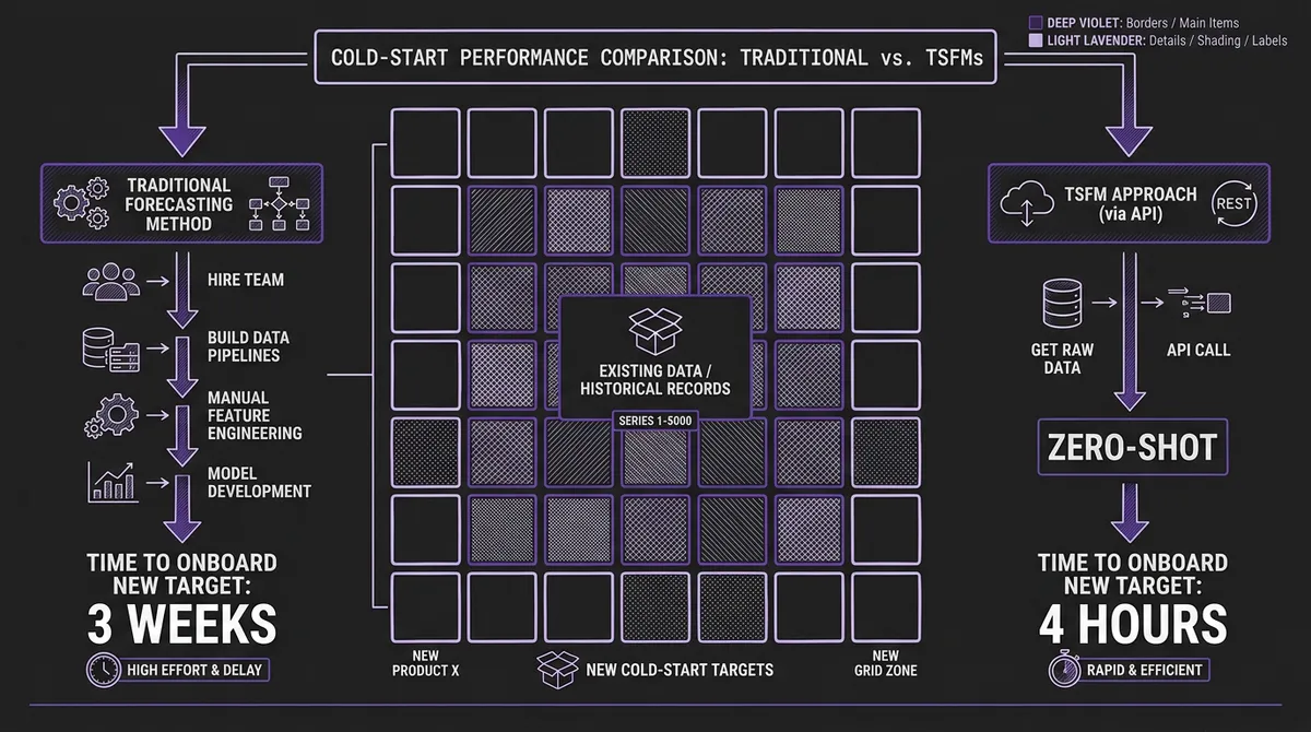
One dimension deserves special attention because it is where the lifecycle cost difference is most dramatic: new forecasting targets.

Traditional systems struggle with cold starts. When a retailer launches a new product, an energy utility expands to a new grid zone, or a logistics company opens a new shipping lane, there is no historical data to train on. The traditional response is some combination of analoging (manually selecting a "similar" existing series to clone), rule-based heuristics, or simply waiting for enough data to accumulate. Our energy demand forecasting case study documented this precisely: onboarding a new grid zone took three weeks with the traditional LightGBM pipeline. Cold-start forecast quality was poor for the first six to twelve months.

TSFMs solve cold starts architecturally. Because the model has learned general temporal patterns during pretraining, it can generate useful forecasts from as few as a dozen observations. New zone onboarding in the energy case study dropped from three weeks to under four hours. Retail demand planning for new product launches goes from "wait and hope" to "forecast from day one."

For organizations that frequently add new forecasting targets — growing retailers, expanding utilities, scaling logistics operations — this is not a marginal improvement. It is a structural advantage that compounds over time.

A Realistic Total Cost Comparison

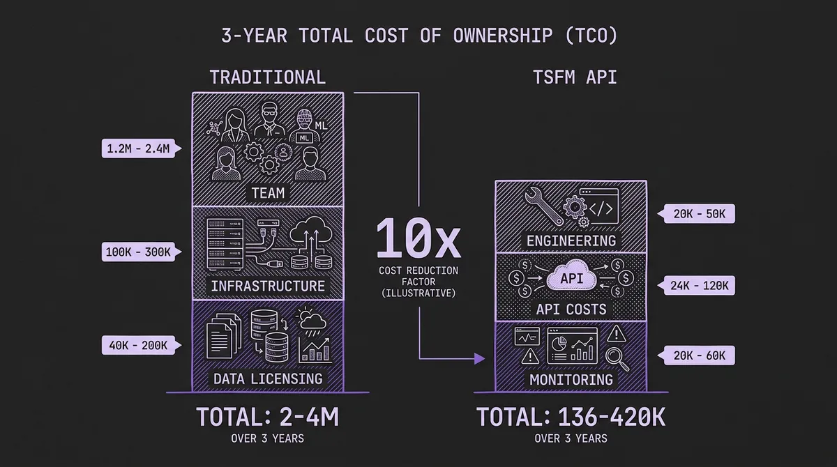
Let us put approximate numbers on both paths for a mid-size enterprise deploying demand forecasting across 5,000 series.

Traditional Pipeline

Category	Year 1 (Build)	Years 2-3 (Maintain)
Team (4-6 FTE)	$600K - $1.2M	$1.2M - $2.4M
Infrastructure (GPU, storage, MLOps tooling)	$50K - $150K	$100K - $300K
Data licensing (weather, economic)	$20K - $100K	$40K - $200K
Opportunity cost (time to production: 6-12 months)	Significant	—
Total (3-year)		$2M - $4.3M

TSFM via API

Category	Year 1	Years 2-3
Engineering integration (1-2 engineers, part-time)	$50K - $100K	$20K - $50K
API usage costs	$12K - $60K	$24K - $120K
Monitoring and evaluation	$10K - $30K	$20K - $60K
Total (3-year)		$136K - $420K

These numbers are illustrative, not universal. Your specific costs depend on data volume, complexity, latency requirements, and team composition. But the order-of-magnitude difference is real and consistent across the deployments we have observed.

When Traditional Methods Still Win

This is not a one-sided argument. There are legitimate scenarios where building a traditional forecasting pipeline is the right choice.

Regulatory requirements for model interpretability. In regulated industries — financial risk, insurance pricing, pharmaceutical demand — regulators may require that you explain exactly how a forecast was generated. Statistical methods like ARIMA and ETS provide transparent, decomposable predictions. Foundation models are black boxes. The 2026 landscape is moving toward better explainability tooling, but it is not there yet.

Extreme domain specificity. If your time series exhibit patterns that are genuinely unlike anything in the foundation model's pretraining corpus — exotic financial derivatives, niche industrial processes with physics-driven dynamics, biological signals with unusual temporal structures — a purpose-built model trained on your domain data may outperform zero-shot inference.

Existing investment. If you already have a mature, well-maintained forecasting pipeline with a stable team, the switching cost may not justify the savings. The strongest case for TSFMs is greenfield: when you are building from scratch or when your existing system has accumulated enough technical debt that replacement is cheaper than remediation.

Data sovereignty. Some organizations cannot send their data to an external API. If your time series contain classified, regulated, or competitively sensitive information, you may need to run inference on-premises. Self-hosted TSFM deployment is possible but reintroduces much of the infrastructure complexity that API-based inference eliminates.

When TSFMs Are the Clear Choice

Conversely, several scenarios make the TSFM path unambiguously better.

You do not have a forecasting team and do not want to build one. If forecasting is a supporting capability rather than a core competency — and for most organizations, it is — spending $2 million to build and staff a forecasting function is difficult to justify when an API can provide 80-90% of the accuracy for 10% of the cost.

You need forecasts across many domains. A single TSFM serves retail demand, energy load, supply chain volumes, manufacturing sensor data, and financial metrics without separate models for each domain.

You need to move fast. If time-to-value matters — and in competitive markets, it always does — going from zero to production forecasts in days rather than months is a strategic advantage. Our energy case study showed 23% accuracy improvement over the legacy pipeline, achieved in a fraction of the implementation time.

You forecast many heterogeneous series. The larger and more diverse your forecasting portfolio, the more the traditional per-series model management burden compounds. TSFMs handle heterogeneity natively because they were pretrained on diverse data. This advantage grows superlinearly with scale.

You have frequent cold starts. Rapidly expanding product catalogs, sensor deployments, or service territories make the cold-start advantage decisive.

What the Benchmarks Actually Show

The evolution of the Makridakis competitions tells a revealing story about where forecasting methodology is heading.

In M3 (2000), statistical methods dominated. Combinations of simple methods often outperformed complex individual models. In M4 (2018), the winner was a hybrid — exponential smoothing fused with a recurrent neural network — but pure ML methods still underperformed statistical baselines. In M5 (2020), pure ML finally won decisively, but required months of feature engineering per competitor.

Now, TSFMs are achieving competitive results with zero-shot inference — no training on the target data at all. Amazon's Chronos-Bolt outperforms commonly used statistical and deep learning models even when those models are trained on the benchmark data. This is not marginal. It is a paradigm shift: competitive accuracy without any of the lifecycle cost described above. For a deeper analysis of how these benchmarks are constructed and what their limitations are, see our post on the challenges of benchmarking TSFMs.

To be fair, the picture is not uniformly favorable. A Nixtla-led study showed that a statistical ensemble (AutoARIMA, AutoETS, AutoCES, DynamicOptimizedTheta) outperformed Chronos by 10-11% on over 50,000 series from M1/M3/M4 datasets. The debate over whether TSFMs truly exhibit "foundational" generalization or remain tied to their pretraining domains continues in the research community. This is why we advocate starting with zero-shot evaluation on your data rather than trusting any single benchmark.

One industry signal worth noting: AWS deprecated its managed Amazon Forecast service in July 2024, directing customers toward foundation-model-based approaches. When a hyperscaler sunsets its own traditional forecasting product, the directional bet is clear.

The Convergence Path

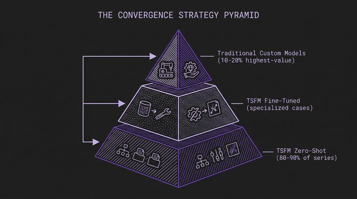
The choice is not always binary. A growing pattern we see among practitioners is convergence: use TSFM zero-shot inference as the default for the majority of forecasting targets, and invest in traditional methods only for the high-value, domain-specific series where the marginal accuracy improvement justifies the engineering cost.

This mirrors how the energy utility in our case study deployed: Chronos-Large as the default for most grid zones, with Moirai-Large for the 30 zones where spatial correlation warranted a more specialized approach. The traditional LightGBM pipeline was not replaced wholesale — it was narrowed to the cases where it uniquely added value, while the foundation model handled everything else.

This convergence strategy lets organizations capture 80-90% of the TSFM cost savings while preserving traditional methods for the 10-20% of series where they genuinely outperform. It also provides a natural migration path: start with TSFMs for new forecasting targets (eliminating cold-start delays), gradually backfill existing targets as confidence grows, and retain traditional models only where they measurably add value.

Getting Started

If you are evaluating whether TSFMs can replace or supplement your existing forecasting infrastructure, the lowest-risk starting point is a parallel evaluation. Run your existing pipeline alongside zero-shot TSFM inference on the same historical data and compare accuracy on held-out periods. Our playground lets you test this interactively with your own data before writing any integration code.

For organizations building forecasting capabilities from scratch, the recommendation is simpler: start with the API. You can always invest in custom modeling later if TSFM accuracy proves insufficient for your highest-value use cases. But the data from production deployments consistently shows that "later" rarely arrives — zero-shot performance is sufficient for the vast majority of enterprise forecasting problems. Review the model catalog to understand what is available, read the quickstart guide, and put your data through the system. The results will speak for themselves.