LoRA and PEFT for Time Series Foundation Models: A Technical Guide

Zero-shot inference is the default way most practitioners use time series foundation models. Hand the model a history window, get a forecast back, no training required. It works remarkably well — well enough that zero-shot TSFMs now dominate leaderboards like FEV Bench and GIFT-Eval. But zero-shot has a ceiling. When your data distribution diverges significantly from the pretraining corpus — clinical vital signs, proprietary sensor telemetry, niche financial instruments — that ceiling becomes visible fast.

The traditional answer is full fine-tuning: update every parameter on your domain-specific data. This works, but it is expensive, prone to overfitting on small datasets, and risks catastrophic forgetting of the general knowledge that made the foundation model useful in the first place. Low-Rank Adaptation (LoRA) offers a middle path: freeze the pretrained weights, inject small trainable low-rank matrices into specific layers, and adapt the model with a fraction of the parameters. The technique has transformed LLM fine-tuning since Hu et al. introduced it in 2021. Its application to TSFMs is newer, less standardized, and — as we will see — architecturally dependent in ways that matter.

This post covers the technical details: which TSFM architectures support LoRA, which layers to target, what rank values to use, how tokenization interacts with adaptation, what the research shows about practical improvements, and where the failure modes hide. We link to all models we host throughout so you can connect theory to available inference endpoints.

The LoRA Mechanism, Briefly

For readers familiar with the technique, skip ahead. For those who want the mechanics:

A pretrained weight matrix W₀ ∈ ℝ^(d×k) is frozen. Two small matrices A ∈ ℝ^(d×r) and B ∈ ℝ^(r×k) are added, where r << min(d, k). During the forward pass, the output becomes:

h = W₀x + BAx

The scaling factor α/r controls the magnitude of the adaptation, where α (lora_alpha) is a hyperparameter. Only A and B are trained. For a layer with d=768 and k=768, full fine-tuning trains 589,824 parameters. With r=8, LoRA trains only 12,288 — a 98% reduction.

At inference time, the LoRA matrices can be merged into the base weights (W = W₀ + BA), adding zero latency overhead. This is a critical property for production deployment: you get the accuracy benefits of adaptation with identical inference cost.

TSFM Architecture Taxonomy for LoRA

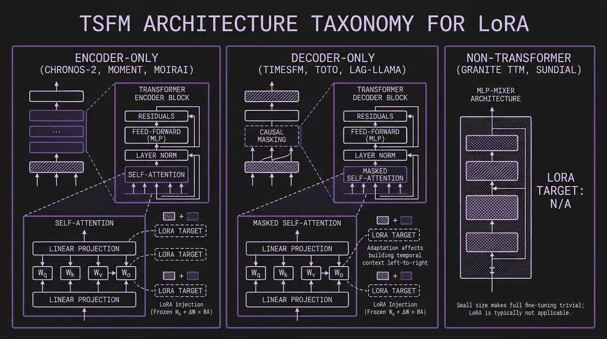
How LoRA applies to a TSFM depends fundamentally on its architecture. The current landscape has three dominant families, each with different adaptation characteristics.

Encoder-Only Models

Examples we host: Chronos-2 (120M), MOMENT (385M), Moirai 2.0 (14M-311M)

Encoder-only TSFMs process the full input sequence through self-attention layers and project the final representations through a task-specific head (forecasting, anomaly detection, classification, imputation). LoRA targets the self-attention projection matrices — Wq, Wk, Wv, Wo — in each transformer block. The task head is typically a lightweight linear layer that is always trainable.

This architecture is the most straightforward for LoRA. The attention matrices capture sequence-level patterns; low-rank adaptation adjusts these patterns toward domain-specific dynamics without disrupting the overall representation structure.

Chronos-2 uses a T5-encoder backbone with two novel attention mechanisms: time attention (self-attention along the temporal axis with RoPE positional encoding) and group attention (cross-attention across related time series for multivariate inputs). LoRA can target either or both mechanisms.

MOMENT is a T5-based encoder where the forecast head is randomly initialized and must be fine-tuned before use. The recommended workflow is linear probing first (freeze encoder, train head), then optionally add LoRA modules for deeper adaptation.

Decoder-Only Models

Examples we host: TimesFM 2.5 (200M), Toto (151M), Timer-XL (84M), Lag-Llama (~10M), Time-MoE (200M active / 2.4B total), Cisco Time Series (500M)

Decoder-only models use causal (autoregressive) attention: each position can only attend to preceding positions. LoRA targets the same Wq, Wk, Wv, Wo matrices, but the causal mask means adaptation affects how the model builds temporal context left-to-right.

For Lag-Llama, which has only 2.4M total parameters, LoRA with r=2 adds roughly 16K trainable parameters — 0.66% of the model. Research from Maizak et al. (2024) showed that even at this tiny scale, LoRA meaningfully improved domain-specific accuracy.

For Time-MoE, the mixture-of-experts architecture introduces a complication: should LoRA adapt the shared attention layers, the expert feed-forward layers, or both? Current research has not systematically studied this. The Time-MoE repository only documents full fine-tuning; LoRA integration would require targeting the attention projections within each transformer block while leaving the expert routing mechanism frozen.

Non-Transformer Architectures

Examples we host: Granite TTM (~1M), Granite TSPulse (~1M), Sundial (128M, flow-matching)

Granite TTM and TSPulse use MLP-Mixer architectures with under 1M parameters. LoRA is not applicable here — the models are already small enough that full fine-tuning is trivial. IBM's granite-tsfm toolkit provides few-shot fine-tuning workflows where TTM reaches competitive accuracy with only 5% of the training data. These models are designed to be adapted, just not via LoRA.

Sundial uses a transformer backbone with flow-matching loss instead of discrete tokenization. LoRA could theoretically target its attention layers, but fine-tuning code is not yet released. The Sundial repository states it is coming soon.

Model-by-Model LoRA Support Matrix

Here is the current state of LoRA and PEFT support across every model we host, based on official documentation, repository code, and published research as of February 2026.

Model	Params	Architecture	Native LoRA	Fine-Tuning	Framework
Chronos-2	120M	Encoder (T5)	Yes	LoRA + Full	AutoGluon
MOMENT	385M	Encoder (T5)	Yes	LP + LoRA + Full	momentfm
Moirai 2.0	14-311M	Encoder (AVA)	Research only	Full	Uni2TS
TimesFM 2.5	200M	Decoder	No	Full + ICF	timesfm
Toto	151M	Decoder	No	Full (limited)	toto
Timer-XL	84M	Decoder	No	Full	OpenLTM
Lag-Llama	~10M	Decoder (Llama)	Research only	Full	GluonTS-style
Time-MoE	200M/2.4B	Decoder (MoE)	No	Full	Time-MoE
Sundial	128M	Transformer + Flow	Pending	Coming soon	OpenLTM
Granite TTM	~1M	MLP-Mixer	N/A	Full (few-shot)	granite-tsfm
TSPulse	~1M	MLP-Mixer	N/A	TSLens module	granite-tsfm
TiRex	~300M	xLSTM	No	Contact vendor	N/A
Chronos-Bolt	48-205M	Direct multi-step	No (inherits Chronos)	Via AutoGluon	AutoGluon
Moirai-MoE	86M/935M	Sparse MoE	No	Via Uni2TS	Uni2TS

"Native LoRA" means the model's official framework includes LoRA as a documented, tested fine-tuning mode. "Research only" means LoRA has been applied in published papers but is not part of the official tooling.

Deep Dive: Chronos-2 LoRA

Chronos-2 has the most mature LoRA integration of any TSFM, built directly into AutoGluon TimeSeries. The default fine-tuning mode is LoRA, not full fine-tuning. Here are the details from the Chronos-2 paper and AutoGluon documentation.

Default Configuration

from autogluon.timeseries import TimeSeriesPredictor

predictor = TimeSeriesPredictor(prediction_length=24)
predictor.fit(
    train_data,
    hyperparameters={
        "Chronos": {
            "model_path": "amazon/chronos-2",
            "fine_tune": True,
            # LoRA defaults:
            "fine_tune_mode": "lora",      # "lora" or "full"
            "lora_r": 8,                    # rank
            "lora_alpha": 16,               # scaling factor
            "learning_rate": 1e-5,
            "max_steps": 1000,
            "per_device_train_batch_size": 32,
        }
    }
)

Architectural Targeting

Chronos-2's encoder has two distinct attention types:

1. Time attention: self-attention along the temporal axis within each variate, using RoPE. LoRA adapts the Wq/Wk/Wv/Wo projections that control how temporal patterns are extracted.

2. Group attention: cross-attention between variates, enabling the model to learn inter-series dependencies. LoRA here adjusts how the model weighs correlations between related series.

By default, AutoGluon applies LoRA to all attention projections in both mechanisms. The tokenization layer — which scales and bins continuous values into a discrete vocabulary of 4096 tokens — is frozen. This means LoRA adapts how the model processes and relates token sequences, but not how raw values map to tokens. If your domain has a radically different value distribution than the pretraining data, this frozen tokenization can be a bottleneck (more on this in the failure modes section below).

When to Use Full Fine-Tuning Instead

AutoGluon documents that full fine-tuning (fine_tune_mode="full") with a lower learning rate (1e-6 vs 1e-5) can outperform LoRA when:

• You have a large, domain-specific dataset (tens of thousands of series)
• The target domain has fundamentally different statistical properties than the pretraining corpus
• You can afford the compute and are willing to manage a larger model artifact

For most practitioners, LoRA is the recommended default. The compute savings are substantial — LoRA trains roughly 0.5% of the 120M parameters — and the risk of overfitting on small datasets is dramatically lower.

Deep Dive: MOMENT LoRA

MOMENT from the CMU Auton Lab has native PEFT support with a distinctive multi-stage workflow designed around the model's encoder-only architecture.

The Three-Stage Workflow

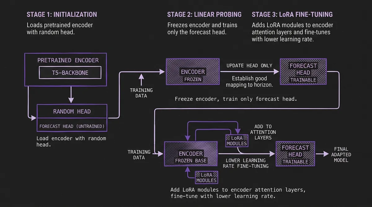
1. Initialization: Load the model with a task-specific head. The encoder weights are pretrained; the head is randomly initialized.

from momentfm import MOMENTPipeline

model = MOMENTPipeline.from_pretrained(
    "AutonLab/MOMENT-1-large",
    model_kwargs={
        "task_name": "forecasting",
        "forecast_horizon": 96
    }
)
model.init()

2. Linear probing: Freeze the entire encoder. Train only the forecast head. This establishes a good mapping from MOMENT's learned representations to your specific forecast horizon and loss function.

3. LoRA fine-tuning: After linear probing converges, add LoRA modules to the encoder's attention layers and continue training with a lower learning rate. This refines the encoder's representations for your domain while preserving the general temporal patterns learned during pretraining.

This staged approach is more involved than Chronos-2's single-step LoRA, but it is motivated by MOMENT's architecture. The forecast head is a lightweight linear projection from patch embeddings of dimension D to the forecast horizon. Without linear probing first, LoRA gradients must simultaneously adapt the encoder representations and train a randomly-initialized head — a harder optimization problem.

MOMENT as a PEFT Research Testbed

MOMENT has become a popular research platform for studying PEFT methods on TSFMs. The TRACE paper (Time SeRies PArameter EffiCient FinE-tuning) used MOMENT-base (12 transformer encoder layers, d=768, 12 attention heads) as its primary testbed. TRACE introduces Gated DSIC (Domain-Specific Importance Coefficients) — a learned gating mechanism that selects which LoRA modules are actually important and prunes the rest. On MOMENT, TRACE reduced the forecast head parameters by 87-98% while matching or exceeding standard LoRA accuracy.

How LoRA Interacts with TSFM Tokenization

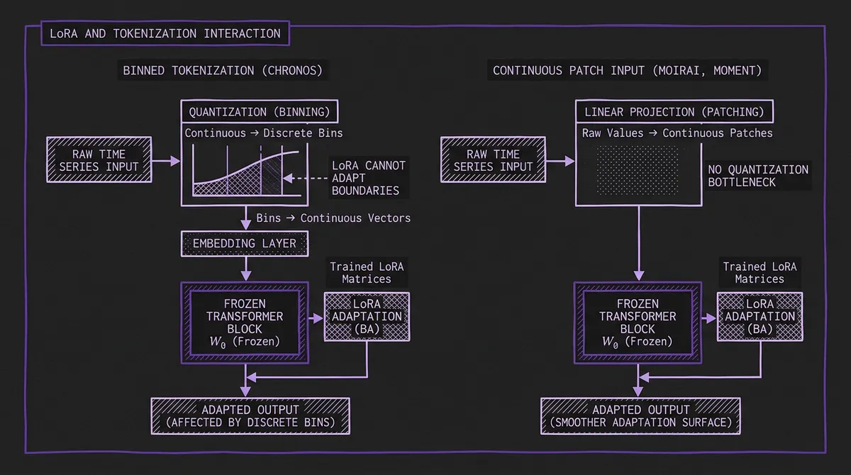
The interaction between LoRA and the model's input processing strategy is a nuanced technical point that is often overlooked. Different tokenization strategies create fundamentally different adaptation surfaces.

Binned Tokenization (Chronos v1, Chronos-2)

Chronos scales input values by their mean absolute value, then quantizes into B uniform bins (B=4096). The result is a sequence of integer token IDs — identical in structure to language model tokens. The embedding layer maps these IDs to continuous vectors, and the transformer processes those vectors.

LoRA operates on the transformer layers, not the tokenization or embedding layer. This means:

• LoRA can adjust how the model relates temporal patterns in the embedded token sequence.
• LoRA cannot adjust the boundaries of the bins themselves. If your domain has a value distribution that is poorly served by the pretrained bin boundaries (e.g., highly skewed distributions, extreme outliers), LoRA cannot compensate for information lost at the quantization stage.
• The mean absolute scaling is applied per-series, so level differences are already handled. LoRA's value is primarily in adapting the model's attention patterns to domain-specific temporal dynamics — recurrence structures, regime change patterns, seasonal profiles — that differ from the pretraining corpus.

The FourierFT paper from NeurIPS 2024 Workshop found that for Chronos Tiny, even 2,400 FourierFT parameters (vs. LoRA's typical ~16K-442K) surpassed SOTA, suggesting that binned tokenization creates a sufficiently robust representational space that very few adaptation parameters are needed.

Continuous Patch-Based Input (Moirai, MOMENT, TimesFM)

Moirai, MOMENT, and TimesFM process time series as continuous-valued patches. A patch of P consecutive values is linearly projected into the model's latent space. There is no quantization bottleneck — the full continuous information is preserved.

LoRA adapts the transformer layers that process these patch embeddings. The input projection layer (a linear map from ℝ^P → ℝ^d) is typically frozen, but since it is a learned linear projection (not a discrete embedding), the model can represent arbitrary continuous values at full precision.

This means LoRA for patch-based models has a smoother adaptation surface. There is no discrete information bottleneck between the raw data and the adapted layers. In principle, this should make LoRA more effective for domain adaptation — and the research from Maizak et al. supports this, showing that LoRA on Moirai maintained competitive accuracy even with very low rank (r=2).

Flow-Matching (Sundial)

Sundial uses neither discrete tokens nor standard patch projections. Its TimeFlow loss is based on flow-matching, where the model learns to transform a simple prior distribution into the target forecast distribution through a learned velocity field. LoRA would target the transformer backbone that parameterizes this velocity field, but the interaction between low-rank adaptation and flow-matching dynamics is entirely unstudied. This is an open research question.

Rank Selection: What the Research Shows

The choice of rank r is the most important LoRA hyperparameter. Too low and the adaptation is too constrained to capture domain-specific patterns. Too high and you lose the regularization benefits and approach full fine-tuning in parameter count.

Empirical Results Across Studies

Study	Model	Rank (r)	Alpha (α)	Trainable Params	Result
Maizak et al.	Lag-Llama, Moirai, Chronos	2	16	16K (Lag-Llama)	Outperformed full FT on 4 of 6 model-metric pairs
NeurIPS '24 Workshop	Chronos (Tiny/Small/Base)	16 (VeRA)	—	2.4K (FourierFT)	FourierFT with 2.4K params beat LoRA with 442K
LLIAM	LLaMA-7B repurposed	8	16	~4M	14.8% of baseline training time
Chronos-2 default	Chronos-2 (120M)	8	16	~600K	Official recommended config
TRACE	MOMENT-base	2 (initial), max 4 (AdaLoRA)	—	Varies (pruned 87-98%)	Matched LoRA with far fewer params
MSFT	Moirai Small/Base	8	16	—	Multi-scale FT outperformed LoRA baseline

Key Takeaways for Rank Selection

r=2 to r=8 is sufficient for most TSFMs. This is strikingly lower than the r=16 to r=64 commonly used for LLM fine-tuning. The likely explanation is model scale: most TSFMs are 10M-400M parameters, where the attention weight matrices are smaller and lower-rank adaptations capture more of the relevant variation. The ablation study in Maizak et al. explicitly tested increasing r and found that performance plateaus quickly, especially for larger models.

Scaling factor α/r matters. The standard configuration of α=16 with r=8 gives a scaling factor of 2.0. With r=2 and α=16, the scaling factor is 8.0 — each adaptation contributes more aggressively. If you use very low rank, consider reducing α proportionally to avoid destabilizing training.

Consider signal characteristics. The NeurIPS 2024 Workshop paper found that LoRA (442K params) outperformed ultra-compact methods on low-variability signals (heart rate), while FourierFT (2,400 params) was superior on high-variability signals (mean blood pressure). If your target series has low noise and regular patterns, even r=2 may suffice. If it has high-frequency noise and irregular dynamics, r=8 is a safer default.

Which Layers to Target

Standard Configuration

The default approach, used in most published research and in Chronos-2's AutoGluon integration, is to apply LoRA to all four attention projection matrices in every transformer layer:

• Wq (query projection) — adapts what the model "asks" about at each position
• Wk (key projection) — adapts what each position "advertises" to others
• Wv (value projection) — adapts what information is retrieved when attention is applied
• Wo (output projection) — adapts how attended information is mixed before the residual connection

Selective Targeting

Not all layers contribute equally to adaptation. The LLIAM paper applied LoRA to only Wq and Wv (queries and values), following the original LoRA paper's finding that these two matrices carry most of the adaptation signal in LLMs. This halves the LoRA parameter count.

TRACE goes further with its Gated DSIC mechanism: start with LoRA on all linear layers, then learn gating coefficients that determine which LoRA modules are important. Unimportant modules are pruned. On MOMENT-base, TRACE found that a 95% mask percentage (pruning 95% of LoRA modules) maintained full accuracy — meaning only 5% of the LoRA modules were doing useful work.

Feed-Forward Layers

Most TSFM LoRA implementations target only attention projections. The feed-forward network (FFN) layers in each transformer block — which typically account for 2/3 of the parameters — are left frozen. This follows standard practice from LLM LoRA, where attention adaptation is sufficient for most tasks.

However, the MSFT paper found that for encoder-based TSFMs like Moirai, their Multi-Scale Fine-Tuning approach (which adapts FFN layers at multiple temporal scales) outperformed attention-only LoRA by a meaningful margin. This suggests that for TSFMs specifically, the FFN layers may play a larger role in encoding temporal scale information than in language models.

Training Hyperparameters

Based on the consolidated research and official documentation:

Parameter	Conservative	Default	Aggressive	Notes
Rank (r)	2	8	16	Higher for noisier signals
Alpha (α)	8	16	32	Keep α/r between 1-4
Learning rate	5e-6	1e-5	3e-4	Chronos-2 default: 1e-5
Optimizer	AdamW	AdamW	AdamW	Standard across all papers
Batch size	16	32	128	Larger for stable gradients
Max steps	500	1000	5000	Chronos-2 default: 1000
LoRA dropout	0	0.05	0.1	Regularization for small datasets
Weight decay	0	0.01	0.1	Standard AdamW decay
Warmup	0	100 steps	10% of total	Helps with stability

Learning rate is critical. Full fine-tuning of TSFMs typically uses 1e-6 to 5e-6. LoRA can tolerate 2-10x higher learning rates because fewer parameters are being updated and the low-rank constraint provides implicit regularization. The catastrophic forgetting paper on TimesFM showed that high learning rates during fine-tuning caused MAE to spike from 0.15 to 1.60 — a 967% degradation on previously learned data. LoRA mitigates this by keeping most weights frozen, but the learning rate still matters.

Data Requirements

One of LoRA's key advantages is efficient use of limited data. Concrete datapoints from the literature:

• 4,020 samples (split 8:1:1) was sufficient for meaningful LoRA adaptation of Chronos and Moirai on ICU vital signs data (Maizak et al.)
• 5% of training data was sufficient for Granite TTM few-shot fine-tuning to approach full-data accuracy (IBM granite-tsfm)
• 1-5 in-context examples improved TimesFM by 6.8% over zero-shot via In-Context Fine-Tuning, without modifying any weights (Google ICF paper)
• 617-1,428 series per dataset was used for LLIAM LoRA on 7 diverse datasets

As a rule of thumb: if you have fewer than 500 series, LoRA with r=2 and aggressive early stopping is likely safer than full fine-tuning. If you have fewer than 100 series, consider zero-shot with conformal calibration as an alternative to any weight-based adaptation.

Practical Results: LoRA vs. Zero-Shot vs. Full Fine-Tuning

ICU Vital Signs (Out-of-Domain Adaptation)

The most comprehensive head-to-head comparison comes from Maizak et al. (2024), which tested LoRA (r=2, α=16) against zero-shot and full fine-tuning on eICU clinical data — a domain not represented in any TSFM's pretraining corpus.

Heart Rate Forecasting (MSE, lower is better):

Model	Zero-Shot	LoRA	Full FT	LoRA vs Zero-Shot
Chronos Tiny	7.37	7.22	9.10	-2.0%
Chronos Small	7.19	7.08	10.04	-1.5%
Lag-Llama	15.55	10.39	16.60	-33.2%

Mean Blood Pressure Forecasting (MSE, lower is better):

Model	Zero-Shot	LoRA	Full FT	LoRA vs Zero-Shot
Chronos Tiny	25.60	19.79	19.90	-22.7%
Chronos Small	25.04	19.89	20.93	-20.6%
Lag-Llama	24.10	23.83	22.93	-1.1%

Two critical observations:

1. LoRA outperformed full fine-tuning in 4 of 6 model-metric combinations. Full fine-tuning on these small clinical datasets caused overfitting — the model fit training noise rather than learning domain-specific patterns. LoRA's low-rank constraint acted as an implicit regularizer.

2. The improvement magnitude varied wildly. Lag-Llama saw a 33% MSE reduction on heart rate but only 1% on blood pressure. Chronos saw the opposite pattern. This is not random — it reflects the interaction between each model's pretrained representations and the target signal's characteristics.

Multi-Scale Fine-Tuning Comparison

The MSFT paper compared LoRA, AdaLoRA, Linear Probing, and Prompt Tuning on Moirai Small (14M) and Base (91M) across multiple datasets. Key findings:

• On the Solar dataset, MSFT achieved a 24.4% CRPS improvement over full fine-tuning for Moirai Base — a massive gain.
• Standard LoRA was competitive but not dominant. AdaLoRA (adaptive rank allocation) slightly outperformed fixed-rank LoRA in most cases.
• Prompt Tuning (prepending learnable tokens) was consistently the weakest PEFT method for TSFMs, likely because time series lack the discrete semantic structure that makes prompt tuning effective in NLP.

Failure Modes and Pitfalls

Catastrophic Forgetting

The most dangerous failure mode. A 2025 study on TimesFM found that sequential fine-tuning (adapting to domain A, then domain B) caused MAE on domain A to increase from 0.15 to 1.60 — a 967% degradation. The model effectively "forgot" domain A when adapted to domain B.

LoRA partially mitigates this because the base weights remain frozen. You can maintain multiple LoRA adapters (one per domain) and merge the appropriate one at inference time. But if you fine-tune the LoRA adapter sequentially across domains, the adapter itself can forget earlier adaptations.

Recommendation: Maintain separate LoRA adapters per domain. Use model routing to select the appropriate base model + LoRA combination at inference time. Never sequentially adapt a single LoRA checkpoint across disparate domains.

Tokenization Bottleneck (Chronos-Specific)

For Chronos and Chronos-2, the binned tokenization layer is frozen during LoRA fine-tuning. If your domain has value distributions that are poorly served by the pretrained bin boundaries — for example, if your series has a bimodal distribution or extreme heavy tails — LoRA cannot compensate for the information lost at quantization.

You can diagnose this by comparing the distribution of your series values against the bin boundaries. If a large fraction of your values cluster into a small number of bins (poor bin utilization), LoRA adaptation of the transformer layers will have less signal to work with. In this case, consider a patch-based model like Moirai or MOMENT where no quantization occurs.

Full Fine-Tuning Degradation on Small Datasets

Multiple studies show that full fine-tuning can degrade performance when the adaptation dataset is small. The Maizak et al. results above show Chronos Small going from 7.19 (zero-shot) to 10.04 (full FT) on heart rate — a 40% degradation. The model overfit to the small clinical dataset and lost its general forecasting ability.

LoRA's low-rank constraint provides regularization that prevents this. With only r×(d+k) trainable parameters per layer, the adaptation must find a compact representation of the domain shift, which inherently limits overfitting. This is why LoRA is the safer default for datasets with fewer than ~10,000 series.

Distribution Shift Limitations

A 2025 analysis found that when fine-tuned on out-of-distribution data (e.g., individual household electricity consumption vs. population-level training data), fine-tuned TSFMs do not consistently beat smaller task-specific models. LoRA reduces the magnitude of this problem but does not eliminate it. If your target distribution is radically different from anything in the pretraining corpus, even adapted foundation models may underperform a purpose-built model trained from scratch on your domain.

Beyond LoRA: Alternative PEFT Methods for TSFMs

LoRA is not the only parameter-efficient approach. Several alternatives have been tested on TSFMs:

FourierFT (arXiv:2409.11302): Represents the adaptation in a Fourier basis rather than a low-rank matrix decomposition. With only 2,400 parameters (vs. LoRA's 442K), FourierFT surpassed LoRA accuracy on Chronos Tiny for high-variability signals. This is an extremely parameter-efficient method that may be particularly suited to time series where the relevant adaptation has periodic structure.

VeRA (Vector-based Random Matrix Adaptation): Uses shared random matrices with per-layer scaling vectors. Tested at r=16 on Chronos variants; competitive with LoRA but less studied.

BitFit: Trains only bias terms in the network. Minimal parameter overhead but limited adaptation capacity. The NeurIPS 2024 Workshop found it inferior to LoRA and FourierFT for TSFMs.

LayerNorm Tuning: Trains only the LayerNorm affine parameters (γ, β). Extremely lightweight but sufficient for mild distribution shifts (e.g., same domain, different statistical properties).

In-Context Fine-Tuning (ICF): Google's approach for TimesFM, where the model is further pretrained with in-context examples separated by a learnable separator token. At inference time, providing a few domain-specific examples improves accuracy by 6.8% without modifying weights. This is not PEFT in the traditional sense, but it achieves a similar goal — domain adaptation with minimal compute — and avoids the catastrophic forgetting problem entirely since no weights are changed at inference time. See the ICF paper for details.

TRACE (arXiv:2503.16991): LoRA with learned importance pruning via Gated DSIC. Starts with LoRA on all layers, learns which modules matter, prunes the rest. Reduces LoRA overhead by 87-98% on MOMENT with no accuracy loss. Training overhead is 1.3x of standard LoRA; inference time is identical.

Practical Recommendations

Based on the research and our experience running these models at scale:

If your data is in-distribution (similar domains, frequencies, and statistical properties as the model's pretraining data): start with zero-shot. Use conformal calibration to fix prediction interval coverage. LoRA is unlikely to provide large gains.

If your data is mildly out-of-distribution (same general domain but different statistical properties): use LoRA with r=4-8 on Chronos-2 (easiest workflow via AutoGluon) or MOMENT (if you need anomaly detection or classification). Budget 1,000-3,000 training steps.

If your data is strongly out-of-distribution (novel domain, unusual statistical properties): consider LoRA with r=8-16 as a starting point, but validate against a simple baseline (seasonal naive, linear regression). If the adapted model does not meaningfully beat the baseline, the domain gap may be too large for LoRA alone. Full fine-tuning of a smaller model like Granite TTM may be more effective.

If you need multi-domain deployment (different LoRA adapters per domain): use Chronos-2 as the base and maintain separate LoRA checkpoints. At inference time, merge the appropriate adapter based on the incoming series' domain. Our model routing system can handle this selection automatically.

If you cannot fine-tune at all (no training infrastructure, no domain data): use TimesFM 2.5 with In-Context Fine-Tuning. Provide a few representative in-context examples at inference time for a lightweight accuracy boost without any weight modification.

What's Next

The PEFT landscape for TSFMs is evolving rapidly. Several directions are actively being researched:

• QLoRA for TSFMs: 4-bit quantization + LoRA has not been formally studied for time series models. Given that most TSFMs are under 500M parameters, the memory savings are less critical than for LLMs, but QLoRA would enable LoRA fine-tuning of models like Cisco Time Series (500M) or Time-MoE (2.4B total) on consumer GPUs.

• LoRA for flow-matching models: As Sundial releases its fine-tuning code, understanding how low-rank adaptation interacts with flow-matching loss will be important. The velocity field parameterization may require different rank and layer targeting strategies than standard attention-based adaptation.

• Mixture-of-LoRA-Experts: Combining MoE architectures like Moirai-MoE with per-expert LoRA adapters could enable fine-grained domain specialization at the expert level.

• Automated rank selection: Current rank choices are manual and based on rules of thumb. Techniques like AdaLoRA (adaptive rank allocation across layers) and TRACE (learned importance pruning) point toward fully automated PEFT configuration — select the model from our catalog, provide your data, and let the system determine the optimal rank, layers, and training duration.

For the latest benchmark results on all models discussed here — including several that support LoRA adaptation — see our benchmarks page and the individual leaderboards for FEV Bench, GIFT-Eval, and BOOM.