TimesFM In-Context Fine-Tuning: Domain Adaptation Without Weight Updates

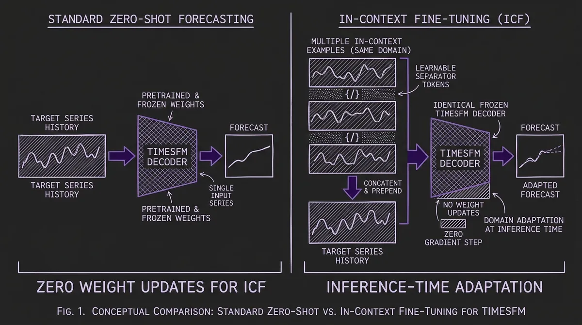
Every time series foundation model faces the same adaptation question: your pretrained model works well on common patterns, but your domain has specific dynamics the model has never seen. The standard answers are full fine-tuning or LoRA, both of which require a training pipeline, labeled data, GPU compute, and ongoing model management. What if you could adapt the model by simply showing it a few examples from your domain — at inference time, with no weight updates at all?

That is exactly what Google Research's In-Context Fine-Tuning (ICF) achieves for TimesFM. Introduced in Faw, Sen, Zhou et al. (2024), ICF extends the few-shot prompting paradigm from large language models to time series forecasting. Instead of only feeding the model the history of the target series, you prepend related time series examples in the context window. The model — specifically pretrained to exploit these examples — adapts to your domain's distribution on the fly.

The results are striking: ICF improves TimesFM's aggregate accuracy by roughly 7% over zero-shot inference on the Monash benchmark suite (with gains up to 25% on individual datasets), and it rivals the performance of explicit fine-tuning on the target domain — without changing a single model weight.

#The Core Idea: Few-Shot Prompting for Time Series

In large language models, few-shot prompting is well understood: you provide example input-output pairs in the prompt, and the model generalizes the pattern to your query. The same principle can be applied to time series, but with important differences.

A standard TSFM takes a single series history as input and forecasts its future:

g: y₁:L → ŷ_{L+1:L+H}

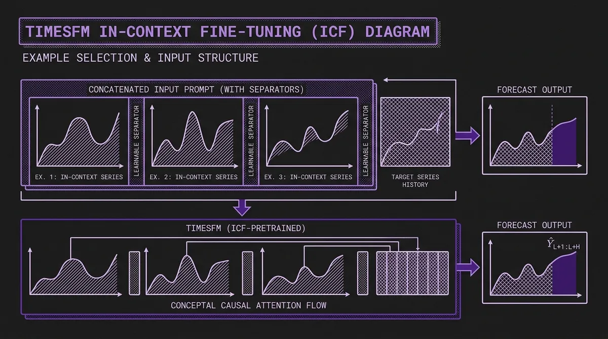
ICF enriches this by prepending n−1 in-context example series from the same domain before the target history:

f: (y⁽¹⁾₁:T₁, y⁽²⁾₁:T₂, ..., y⁽ⁿ⁻¹⁾₁:Tₙ₋₁, y₁:L) → ŷ_{L+1:L+H}

The in-context examples are separated by learnable separator tokens — special embeddings injected between each example series. These separators serve the same role as delimiters in structured LLM prompts: they tell the model where one example ends and the next begins. Without separators, naïvely concatenating multiple series creates ambiguity. For instance, three linear trends concatenated without delimiters can look like a single triangular wave, confusing the model's pattern recognition.

This separator mechanism is critical. The ICF paper demonstrates that concatenation without separators actually degrades performance below zero-shot baselines, while the same examples with separators produce substantial gains.

#How ICF Is Trained

ICF is not a trick you can apply to any existing TSFM. The foundation model must be specifically pretrained to exploit in-context examples. The training procedure modifies the standard decoder-only pretraining in two key ways.

#Multi-Example Pretraining

During pretraining, each training task is constructed by sampling a random number of related time series (from the same dataset) and concatenating them with separator tokens before the target series. The model learns to:

1. Identify that the pre-separator segments are demonstration examples, not part of the target history.
2. Extract distributional patterns (trend shapes, seasonality, noise levels, scale) from the examples.
3. Apply those patterns when forecasting the target series that follows.

The number of in-context examples varies between 0 and n−1 per training task, so the model learns to be useful with any number of examples — including zero, which reduces to standard zero-shot forecasting. This means a single ICF-trained model handles both zero-shot and few-shot inference without separate checkpoints.

#Architecture Foundation

ICF builds on the TimesFM architecture: a decoder-only transformer with input patching (patch size 32), output patching (patch size 128), and stacked causal attention layers. The key architectural requirements are:

• Causal (decoder-only) attention: Each token can attend to all preceding tokens, which means the target series naturally attends to all in-context examples that precede it. Encoder-only architectures like MOMENT use bidirectional attention and would need modifications to support directional ICF, though some models (like Chronos-2) have already introduced group attention mechanisms to handle multi-series in-context learning natively.

• Sufficient context length: The in-context examples consume context window space. TimesFM 2.5 offers a 16,384-step context window, which provides substantial room for both examples and target history. However, note that the ICF capability requires a specifically pretrained TimesFM-ICF checkpoint (created via continued pretraining with separator tokens and multi-example tasks) — the standard public TimesFM 2.5 release does not document ICF prompting support. Earlier TimesFM versions (512 or 2,048 steps) are more constrained in context budget.

• Learnable separator embeddings: Trained alongside the rest of the model, these embeddings mark boundaries between series in the concatenated input.

#Benchmark Results

The ICF paper evaluates on the Monash Forecasting Archive and long-horizon benchmarks (the four ETT datasets and Weather), comparing against statistical baselines (ARIMA, ETS), supervised deep learning models (DeepAR, PatchTST), zero-shot TSFMs, and explicitly fine-tuned TSFMs. Note that Electricity and Traffic are excluded from the zero-shot long-horizon evaluation because they overlap with the pretraining data.

#Key Findings

ICF vs. zero-shot TimesFM: On the Monash benchmark suite, ICF achieves an aggregate scaled MAE of 0.643 versus 0.694 for base TimesFM — roughly a 7% improvement overall. Individual dataset gains range higher (up to ~25% on specific datasets where the target distribution diverges most from the pretraining data), but the headline aggregate improvement is in the single digits.

ICF vs. explicit fine-tuning: ICF performance rivals fine-tuned TimesFM on several benchmarks, despite requiring zero gradient updates. On some datasets, ICF actually slightly exceeds fine-tuning performance — likely because fine-tuning on small target datasets risks overfitting, while ICF leverages the pretrained model's full generalization capacity.

ICF vs. supervised baselines: ICF-prompted TimesFM outperforms dataset-specific DeepAR, PatchTST, and statistical methods on the majority of evaluated benchmarks, while requiring no dataset-specific training.

Scaling with examples: Performance generally improves as more in-context examples are added. The paper's appendix tables show continued gains from 1 up to 50 examples on several benchmarks (including ETT and the Monash aggregate), so the relationship between example count and accuracy does not plateau as quickly as one might expect. That said, even a single in-context example provides a meaningful boost over zero-shot.

#The Adaptation Spectrum

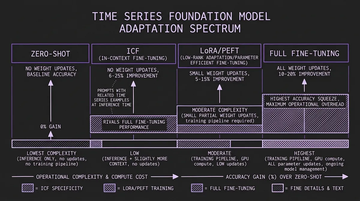
ICF fills a specific gap in the adaptation spectrum. Here is how the available approaches compare:

Approach	Weight Updates	Training Pipeline	Compute Cost	Forgetting Risk	Typical Improvement
Zero-shot	None	None	Inference only	None	Baseline
ICF	None	None	Inference only (slightly more context)	None	~7% aggregate on Monash (up to 25% per-dataset)
LoRA/PEFT	Small subset	Required	Low (minutes on 1 GPU)	Low	5–15% over zero-shot
Full fine-tuning	All parameters	Required	Moderate to high	High	10–20% over zero-shot

The striking property of ICF is that it delivers accuracy gains comparable to parameter-efficient fine-tuning — but with zero operational overhead. There is no training step, no checkpoint management, no risk of catastrophic forgetting, and no need to retrain when your data distribution shifts. You simply change the examples you pass at inference time.

#Practical Implementation

#Selecting In-Context Examples

The choice of in-context examples matters. The ICF paper shows that examples from the same domain as the target series produce the best results. Concretely:

• Same dataset, different series: If you are forecasting one highway's traffic, use traffic data from other highways. If you are forecasting one product's demand, use demand data from related products.
• Same temporal characteristics: Examples should share the target's general frequency and seasonality structure. Using weekly retail data as examples for millisecond sensor data is unlikely to help.
• Diverse within domain: Select examples that cover the range of patterns in your domain rather than picking the most similar series. Diversity helps the model learn the distribution, not just one specific shape.

#Context Window Budget

Each in-context example consumes context window space. With a 16,384-step window and a target history of, say, 1,024 steps, you have approximately 15,000 steps available for examples. At 512 steps per example, that allows roughly 29 examples. The paper's results show continued improvements up to 50 examples on several benchmarks, so using more examples when the context budget allows is generally beneficial.

For older TimesFM versions with shorter context windows, the budget is tighter. TimesFM 2.0 (2,048 steps) allows perhaps 1–3 examples plus a reasonable target history. This is one reason why the progression to longer context windows in TimesFM 2.5 is particularly valuable for ICF.

#Inference Cost

ICF increases inference cost proportionally to the additional context length. If you add 3 examples of 512 steps each, you are processing 1,536 extra time steps through the transformer. For TimesFM's 200M parameter model, this is a modest cost — seconds on a modern GPU. The cost is far lower than any training-based adaptation approach, though note that standard transformer self-attention scales quadratically with total context length, so very large numbers of long examples will increase cost accordingly.

#When to Use ICF

ICF is most valuable in scenarios where:

1. You have related series but limited data per series. ICF shines when you have many short series from the same domain. Instead of trying to fine-tune on small samples (which risks overfitting), you use those samples as in-context examples.

2. The target distribution shifts over time. In streaming inference scenarios where the data distribution evolves, fine-tuned models become stale. ICF adapts instantly — just update the examples to reflect recent data.

3. You need rapid deployment. ICF requires no training pipeline. If you can call the model's inference API and structure your input correctly, you are done. This makes it ideal for prototyping and evaluation.

4. Operational simplicity is paramount. In enterprise settings where managing fine-tuned model versions is costly, ICF eliminates an entire class of operational complexity.

ICF is not the right choice when:

• You have abundant training data and maximum accuracy justifies the engineering cost — explicit fine-tuning or LoRA will squeeze out more performance.
• Your target domain's patterns are extremely far from any time series data (e.g., highly specialized scientific signals) — the model may need deeper weight-level adaptation.
• You are using a model that was not pretrained with ICF support — standard TimesFM or other TSFMs without ICF pretraining will not benefit from in-context examples in the same way.

#ICF in the Broader TSFM Landscape

In-context fine-tuning represents a broader trend in time series foundation models: the convergence with LLM capabilities. Just as LLMs evolved from pure zero-shot models to systems that support few-shot prompting, instruction following, and retrieval-augmented generation, TSFMs are beginning to support analogous adaptation mechanisms.

The ICF approach as described in the paper is specific to decoder-only architectures with causal attention — the same family that includes TimesFM, Toto, Lag-Llama, and Timer. Encoder-only models like MOMENT use bidirectional attention, which means in-context examples would attend to the target series (and vice versa) rather than providing a directional conditioning signal. However, some encoder-based models have already developed their own multi-series conditioning approaches: for example, Chronos-2 uses group attention to handle in-context learning across related series and covariates natively within its encoder architecture.

For now, if you are using TimesFM and want to push beyond zero-shot accuracy without building a training pipeline, ICF is the most operationally efficient path available. As context windows continue to grow across the TSFM ecosystem, expect in-context adaptation to become a standard capability rather than a research novelty.

You can explore TimesFM and other models through the TSFM.ai model catalog and playground, and find the full technical details in the ICF paper and the TimesFM GitHub repository.