CoRA: A Plug-and-Play Adapter for Adding Cross-Channel Correlation to Any TSFM

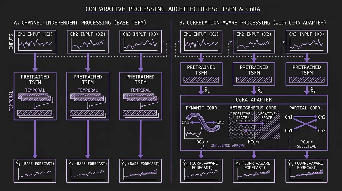
Many recent time series foundation models use channel-independent or single-series formulations that prioritize temporal generalization over explicit cross-channel modeling. In these designs — used explicitly by models such as Timer and Time-MoE — each variate in a multivariate series is treated as a separate single-channel sequence and processed in isolation. The model produces a per-channel forecast without ever seeing two channels simultaneously.

This is not an oversight. Channel-independent modeling is a deliberate design choice that enables TSFMs to generalize across domains: a model that never assumes cross-variate structure will not be misled by it when it does not exist. The trade-off is that it also cannot exploit it when it does. For large swaths of real-world multivariate data — energy grids where supply and demand are coupled, retail portfolios where related SKUs move together, cloud infrastructure where CPU and memory utilization co-evolve — the cross-channel signal is the signal.

CoRA (Correlation-aware Adapter), an ICLR 2026 poster from East China Normal University and Huawei Noah's Ark Lab (arXiv v1: March 23, 2026), adds a lightweight adapter during fine-tuning to recover cross-channel structure without re-pretraining the backbone. It captures three distinct types of cross-channel correlation — dynamic, heterogeneous, and partial — and fuses correlation-aware corrections on top of the TSFM's base predictions, with inference overhead that scales linearly in the number of channels rather than quadratically.

The paper evaluates CoRA across six TSFMs and ten benchmark datasets in a 5% few-shot setting. CoRA lowers averaged MSE on every model–dataset pair in Table 1.

#The Gap: What Channel-Independent Models Miss

The case for channel-independent modeling is compelling. The PatchTST paper showed that channel-independent patch-based models often outperform channel-mixing architectures on standard academic long-horizon benchmarks. iTransformer, which inverts the transformer to run attention across variate tokens rather than time tokens, does model cross-variate structure — but it is an end-to-end architecture, not an adapter that can be layered onto a pretrained TSFM. If adding cross-variate attention to a supervised baseline often degrades benchmark performance, the argument for baking it into a pretrained universal model gets harder to make.

The answer is dataset-dependence. Standard long-horizon forecasting benchmarks (ETT, Exchange Rate, ILI) have relatively weak cross-channel dependencies — the variates are often selected specifically to be structurally similar. Real production datasets — traffic networks, retail demand across a product catalog, multi-node cloud metrics, air quality measurements across a city — frequently exhibit strong, structured, and time-varying cross-channel relationships. On these datasets, ignoring correlations leaves accuracy on the table.

The few TSFMs that do model cross-variate structure have not solved the problem comprehensively. Granite TTM uses an MLP-based channel mixing step, but MLP weights are time-invariant — they cannot adapt to correlations that change over the forecast horizon. Moirai's Any-Variate Attention assigns attention scores across channels, but it does not explicitly distinguish between positive and negative correlations, or between correlations that apply to all channel pairs versus correlations that exist only between specific pairs (e.g., competitor pricing versus supplier pricing within a retail forecast).

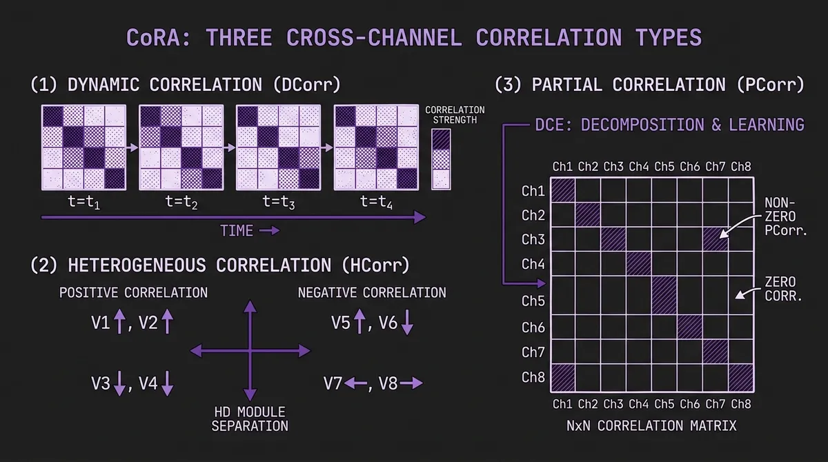
CoRA's authors identify three distinct correlation types that together capture what these methods leave out:

Dynamic Correlation (DCorr): Correlation strength between channels varies over time. The relationship between advertising spend and sales may be strong during a campaign period and nearly zero at other times. A model that learns a fixed correlation matrix will either miss the dynamic signal or overfit to irrelevant periods.

Heterogeneous Correlation (HCorr): Some channels are positively correlated (one going up when another does), others are negatively correlated (one going up when another goes down). Treating these as instances of the same "correlation" concept and mixing them together in a shared representation space conflates genuinely distinct dependency structures.

Partial Correlation (PCorr): Correlations exist only between some channel pairs, not all. Forcing every channel to interact with every other channel introduces noise. In a 321-channel electricity dataset, most pairs of meters are structurally unrelated — aggressively mixing all of them degrades the signal from the few pairs that are genuinely coupled.

#Architecture: DCE, HD, and HPCL

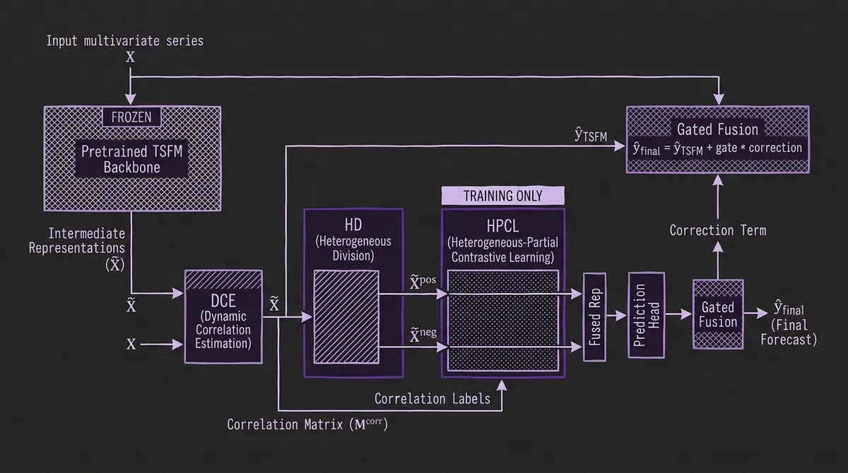
CoRA sits between a pretrained TSFM and its prediction head. During fine-tuning, it reads both the input series X and the TSFM's intermediate latent representations X̃, produces correlation-aware corrections, and gates these corrections with the TSFM's base predictions to produce the final forecast. Three modules handle the three correlation types:

#Dynamic Correlation Estimation (DCE)

DCE produces a per-timestep correlation matrix M^corr ∈ ℝ^{N×N} (where N is the number of channels). Rather than learning this full NxN matrix directly — which would have O(N²) parameter complexity — DCE decomposes the learnable part into two low-rank components:

• A Time-Varying component Q_t ∈ ℝ^{N×M} (with M ≪ N) that captures correlations that change over time. This component is parameterized as a learnable polynomial: the time-varying weights are estimated by a lightweight MLP applied to the TSFM's representations, and polynomial basis functions capture trend and periodic patterns in how correlations evolve. A 3rd or 4th order polynomial is typically sufficient.

• A Time-Invariant component V ∈ ℝ^{M×M} that captures stable, persistent dependencies. This component is learned as a global parameter from randomly initialized learnable vectors, analogous to the self-learned adjacency matrices used in graph neural networks for time series.

The final correlation matrix is the sum of a rule-based Pearson correlation prior (computed directly from the input) and the learned components: M^corr = R + Q_t V Q_t^T. Initializing from Pearson correlation gives DCE a meaningful starting point without requiring many training samples to bootstrap.

#Heterogeneous Correlation Division (HD)

The DCE matrix M^corr contains both positive entries (channels that move together) and negative entries (channels that move inversely). HD separates these into two spaces. Using a Squeeze-and-Excitation mechanism, it applies two separate channel-aware projection layers to the TSFM's latent representations — one projecting into a positive correlation space X̃^pos and one into a negative correlation space X̃^neg. The channel weights are computed adaptively from the representations, so the projection is context-sensitive: a channel that is normally positively correlated with its neighbors will be projected differently during a period where its behavior inverts.

This separation is necessary because the contrastive learning that follows (HPCL) treats positive and negative correlations with opposite objectives. Mixing them before contrastive learning would create conflicting gradients.

#Heterogeneous-Partial Contrastive Learning (HPCL)

HPCL is the component that handles partial correlation — the fact that most channel pairs in a large multivariate dataset are not meaningfully related. It does this through a novel contrastive loss applied separately in the positive and negative spaces.

Using the DCE matrix M^corr as labels, HPCL defines positive pairs (channels with high positive correlation) and negative pairs (channels with low or no correlation) within the positive space, and the analogous split within the negative space. The contrastive loss pulls representations of positively-correlated channel pairs together and pushes unrelated channel pairs apart. Critically, this separation is based on the learned, data-driven correlation matrix from DCE — not a fixed graph structure that must be pre-specified.

Crucially, the contrastive loss in HPCL is training-only. At inference, CoRA still uses its learned projection/fusion path (the HD modules remain active), while the contrastive loss computation itself is skipped. This means inference remains linear in channel count: the dominant overhead is the DCE matrix computation and the final fusion step, not a quadratic attention over channels.

#Heterogeneous Fusion and Gated Output

After HPCL, CoRA fuses the positive and negative correlation representations and passes them through a prediction head to produce a correction term. This correction is added to the TSFM's base prediction via a learned gating scalar:

ŷ_final = ŷ_TSFM + gate * correction

The gating ensures that if CoRA's correction is unreliable (e.g., very early in fine-tuning), the model naturally falls back to the TSFM's base forecast. It also allows the two signal sources to be weighted differently across datasets.

#Benchmark Results

The paper evaluates CoRA in a 5% few-shot fine-tuning setting: the adapter and TSFM are fine-tuned together on 5% of the training set, then evaluated on the full test set. Forecasting horizons H ∈ {96, 192, 336, 720} are averaged. The following MSE values are from Table 1 of the paper:

Dataset	GPT4TS	+CoRA	Timer	+CoRA	TTM	+CoRA
ETTh1	0.468	0.456	0.444	0.432	0.405	0.397
ETTh2	0.375	0.362	0.356	0.350	0.343	0.340
ETTm2	0.279	0.269	0.262	0.257	0.259	0.254
Electricity	0.208	0.201	0.241	0.236	0.179	0.177
Traffic	0.441	0.431	0.456	0.447	0.486	0.481
Weather	0.254	0.245	0.241	0.236	0.226	0.224
AQShunyi	0.850	0.831	0.734	0.724	0.700	0.689

CoRA also improves CALF, UniTime, and MOMENT across all tested datasets. The gains are consistent but vary by dataset: the largest improvements appear on datasets with strong cross-channel dynamics (AQShunyi, Traffic, ETTh1) and smaller improvements on datasets with weaker inter-series structure (ETTm1, ETTm2).

A notable comparison is between TTM's native channel-dependent (CD) mode and a channel-independent TTM (CI) augmented with CoRA. The CoRA-augmented CI version outperforms the native CD version, which suggests that CoRA's explicit three-type correlation modeling is more effective than TTM's built-in MLP-based channel mixing even though both use similar fine-tuning data.

#Ablation: Which Component Contributes What

The paper's ablation (Table 2, ETTm2 dataset, GPT4TS backbone) decomposes the contribution of each CoRA component. Starting from the base TSFM at MSE 0.279: adding HPCL with naive replacements for both DCE and HD brings the MSE to 0.277. Adding the proper DCE module on top of that gives 0.274; adding HD on top gives 0.273. Full CoRA — all three modules together — reaches 0.269. Each component is incremental and all three are necessary to realize the full improvement.

#Comparison With Other Correlation Plugins

The paper also compares CoRA with two existing correlation plugins: LIFT (which exploits leading indicator relationships) and C-LoRA (channel-aware low-rank adaptation). In the 5% few-shot setting on ETTm2, Weather, and Electricity, both plugins degrade the performance of the base TSFM in this limited data regime. The paper attributes this mainly to a mismatch with few-shot TSFM fine-tuning rather than to a universal flaw in those methods — C-LoRA in particular is designed to be trained with an end-to-end backbone from scratch, a different regime from fine-tuning a pretrained model on 5% of data.

This distinction matters for practitioners. LoRA-based TSFM adaptation for temporal domain adaptation generally works well with small amounts of domain data, but adding cross-channel modeling on top of it requires a method that bootstraps effectively from few samples. CoRA's initialization from Pearson correlation and its polynomial-based dynamic modeling are specifically designed for this regime.

#Efficiency

CoRA's inference cost is nearly identical to the base TSFM. The paper measures training time (per epoch) and inference time across three datasets of increasing channel count:

Dataset	Channels (N)	Inference overhead
ETTm2	7	Negligible
Weather	21	Negligible
Electricity	321	Negligible

The linear complexity of the correlation matrix computation (O(N·M) rather than O(N²), where M is the rank hyperparameter) means that even the 321-channel Electricity dataset does not produce a measurable inference slowdown. This is in contrast to attention-based cross-channel methods, which scale quadratically in the number of channels and become expensive at N > 100.

#Low-Data Robustness

A specific concern with any adapter trained on small amounts of domain data is variance: does it actually help at 3% of training data, or does the limited signal result in a noisy adapter that adds noise? The paper evaluates TTM and CALF with CoRA at 3%, 5%, 10%, and 20% of training data on ETTm2 and Weather. CoRA improves TTM even at 3% (0.263 → 0.261 on ETTm2, 0.237 → 0.234 on Weather) — modest, but directionally consistent. Gains compound as data volume increases.

#Practical Deployment

CoRA is available at github.com/decisionintelligence/CoRA. The paper evaluates it on six TSFMs (GPT4TS, CALF, UniTime, MOMENT, Timer, TTM); the repository includes training and evaluation scripts for these backbones. Extending it to other TSFMs requires hooking into the intermediate representation at one or more transformer layers — a forward hook or subclassed module is typically sufficient.

The fine-tuning procedure is straightforward:

1. Load a pretrained TSFM. Use the pretrained weights as initialization; you are not re-pretraining from scratch.
2. Attach CoRA. Instantiate the DCE, HD, and HPCL modules and register a hook to extract the TSFM's intermediate representation at the desired layer.
3. Fine-tune jointly. Train TSFM + CoRA together on your downstream multivariate dataset. The paper uses 5% of available training data; even 3% produces improvements.
4. Evaluate. At inference time, CoRA runs in its forward mode without contrastive learning. The only overhead is the DCE matrix computation and the fusion step.

The sensitivity analysis in the paper suggests K is robust — 3 or 4 are common choices — and that M does not need to scale aggressively with channel count. Default settings in the paper's experiments work well without dataset-specific tuning.

#Situating CoRA in the Adaptation Landscape

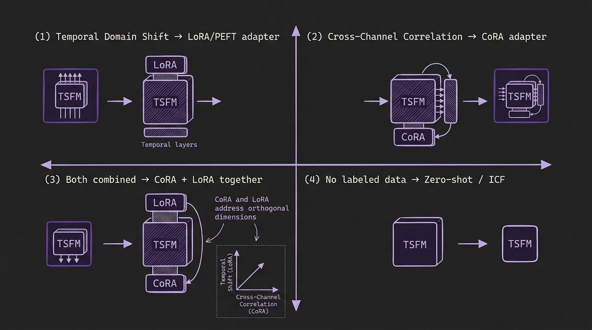
It is worth being precise about what CoRA solves versus what related methods solve, since the surface-level descriptions overlap:

Adaptation need	Recommended approach
Temporal domain shift (new patterns not in pretraining)	LoRA or PEFT; ICF for TimesFM
Cross-variate correlation (channels you want to couple)	CoRA
Both at once	CoRA + LoRA jointly (CoRA handles cross-channel; LoRA handles temporal)
No labeled data at all	Zero-shot TSFM; ICF for TimesFM if in-context examples available

CoRA requires at least a small amount of labeled multivariate data from your target domain. It also requires that the channels you want to correlate are present in that data and are consistently measured. It will not help if your channels are completely unrelated, or if you are doing univariate forecasting. The clearest signal that CoRA will help is when your domain includes groups of channels that are structurally coupled — whether that's by geography (nearby sensors), by causality (lead-lag relationships between supply and demand), or by product hierarchy (parent-child SKU relationships).

Note that for practitioners who use TSFM predictions to drive downstream decisions — pricing, dispatch, inventory replenishment — CoRA's improvements in multivariate accuracy translate directly to better decisions in cases where the decision depends on the relative forecasts of multiple channels. If you are optimizing allocation across a portfolio of assets, having a model that understands the cross-asset dynamics is worth the additional fine-tuning cost.

For teams concerned about the cost of building and maintaining enterprise forecast pipelines, CoRA fits the TSFM-centric paradigm: you still train once (the foundation model), maintain one base model, and use lightweight fine-tuning adapters for domain-specific adjustments. CoRA adds a second dimension of adjustment — spatial (cross-channel) rather than temporal — without requiring a separate model per domain.

#Limitations

No zero-shot cross-channel generalization. CoRA is fine-tuned on the target domain. Unlike the pretrained TSFM backbone, CoRA does not transfer its learned correlation structure to unseen domains. If you switch to a completely different dataset, you need to re-fine-tune CoRA (though the backbone remains fixed).

Channel set must be fixed at fine-tuning time. The DCE module's correlation matrix and the HD projections are sized to the number of channels N in the fine-tuning dataset. Adding or removing channels at inference time requires re-fine-tuning. This is a limitation shared with all correlation-modeling approaches.

Performance on weakly-correlated benchmarks is modest. On ETTm2, which has relatively weak cross-channel structure, CoRA's gain over TTM is 0.259 → 0.254 — real but small. The practical value of CoRA scales with the strength of cross-channel dynamics in your domain. For domains where channels are genuinely independent, there is little reason to add it.

Code coverage is limited to six base TSFMs. The current repository covers GPT4TS, CALF, UniTime, MOMENT, Timer, and TTM. Moirai-MoE, TimesFM, Chronos-Bolt, and other widely-used TSFMs are not yet supported out of the box. Implementing the intermediate representation hook for a new backbone requires some familiarity with that model's forward pass architecture.

#Conclusion

Channel-independent pretraining gives TSFMs their cross-domain generalization, but it leaves cross-channel signal on the table at deployment time. CoRA provides a clean and practical way to recapture that signal: attach a lightweight adapter, fine-tune on a small amount of downstream multivariate data, and get consistent improvements across a broad range of base models and benchmark datasets.

For practitioners building multivariate forecasting systems on top of pretrained TSFMs, CoRA's key practical properties are: (1) it is model-agnostic — the same adapter design works across different TSFM architectures; (2) it is data-efficient — improvements appear even at 3% of training data; (3) it is inference-efficient — linear complexity in channel count with negligible overhead in practice; and (4) it addresses a qualitatively different limitation from LoRA and ICF, so it can be combined with those methods rather than replacing them.

As TSFMs expand into domains where multivariate cross-channel dynamics are the core forecasting challenge — grid balancing, portfolio management, logistics networks — techniques like CoRA that add correlation awareness without sacrificing the zero-shot pretraining base are likely to become a standard part of the deployment toolkit.

---

Primary sources: CoRA arXiv paper (2603.21828) · CoRA OpenReview (ICLR 2026) · CoRA GitHub repository