t0-beta: A 256M Forecasting Model Built for Covariate Context

The Forecasting Company has released t0-beta, a 256-million-parameter forecasting model that follows its 102-million-parameter t0-alpha. The release matters because it treats the information surrounding a target series as part of the forecasting problem. Historical measurements, related variables, and inputs known over the forecast horizon can contribute to a prediction.

For a demand forecast, that context might include promotions and opening hours. For an electricity forecast, it might include calendar effects and a weather forecast available at the decision cutoff. The practical question is whether a model can use those inputs correctly, consistently, and without accidentally seeing the future.

Our guide to forecasting covariates explains that distinction. t0-beta gives practitioners another model to evaluate when a univariate history alone leaves useful information on the table. Its release also offers a useful reminder: model weights, runtime behavior, benchmark configuration, and execution provider all belong in an evaluation record.

#What Changed From t0-alpha

The launch comparison reports improvements over alpha in both probabilistic and point forecasting. These are the authors' results, with a defined comparison scope, rather than measurements performed by TSFM.ai.

Authors' launch comparison	t0-alpha	t0-beta
Parameters	102M	256M
GIFT normalized CRPS, lower is better	0.4941	0.4738
GIFT MASE, lower is better	0.7240	0.6865
FEV skill, higher is better	42.2%	46.7%

The launch positions beta against zero-shot checkpoints. An ensemble, an agent that searches over models, and a fine-tuned forecasting system answer different questions. Their scores can be interesting, but they should not silently become interchangeable with the checkpoint comparison above.

That distinction affects how to read a rank claim. A model can rank highly within a release comparison while a broader, changing leaderboard contains additional systems. Our benchmark directory keeps those benchmark contexts visible. When selecting a model, use the task-level results that resemble your workload, then run a chronological evaluation on your own data.

The increase in parameter count is straightforward. Its effect on your application is not. A larger checkpoint may improve predictions while increasing memory requirements and latency. Whether that trade is worthwhile depends on how many series you forecast, how often you refresh them, and what a missed decision costs operationally.

#Context Is Part of the Model Interface

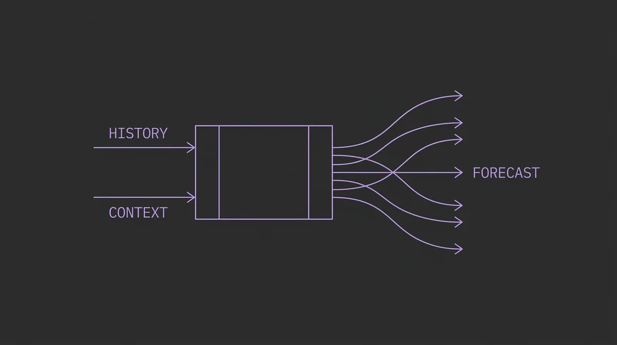
Separate information observed in the past from information available over the prediction horizon.

The t0-beta model card describes a patch-based Transformer with alternating attention over time and variates. It provides probabilistic outputs through 21 native quantiles. Public weights carry an Apache 2.0 license.

The forecasting contract is broader than a single vector of target values. Related histories can be grouped so the model receives joint context, and future-known inputs have their own place in the request. That creates more opportunities to represent a real decision, along with more opportunities to construct an invalid evaluation.

Consider a forecast issued every morning. Yesterday's measured temperature is a historical input. Tomorrow's actual temperature is unavailable. A weather prediction issued before the forecasting cutoff can be a valid future input. Those three values may share a column name in a warehouse, but they have different availability semantics.

The same issue appears in retail. A scheduled promotion may be known several weeks ahead. Realized foot traffic is usually observed afterward. A pipeline that joins both using event dates alone can make the model appear unusually accurate while handing it information the operator could never possess.

A useful input audit starts with the forecast issuance timestamp. For each feature, record when its value first became available, whether later revisions occur, and which vintage the evaluation uses. Then build training and test windows from that availability record. This work often matters more than a small difference between aggregate benchmark scores.

Joint context also requires meaningful grouping. Related stores, neighboring sensors, and unrelated product lines should not automatically receive the same grouping policy. Compare a domain-informed grouping with a simpler baseline and check whether gains hold across the difficult series, rather than only in the average.

#A Covariate Benchmark Is Not Automatically an Ablation

The t0 technical report develops the family's use of time and variate attention and its pretraining approach. For practitioners, the important interpretation is how contextual inputs interact with the evaluation protocol.

A comparison between a covariate benchmark and a benchmark without covariates is not necessarily a controlled experiment. If their datasets, horizons, or scoring rules differ, a change in aggregate score can have several causes. Calling that change the isolated benefit of covariates would overstate what the experiment demonstrates.

A better application-level test holds the task fixed. Use the same target, forecast cutoffs, horizons, and scoring code. Run the model with target history alone, then add historical context, then add inputs available over the horizon. Compare all three against a seasonal baseline under the same evaluation windows.

This approach answers an actionable question: which information improves this decision? It can reveal a useful covariate that helps only during holidays, an unreliable input that degrades performance during outages, or a feature whose apparent benefit disappears once leakage is removed.

For probabilistic predictions, also inspect interval coverage. Lower average point error does not ensure that uncertainty intervals have useful calibration. Measure coverage and width across operating regimes, especially the periods when the forecast informs a consequential response.

#Run It With the Matching Runtime

The first-party runtime and model card document how to load the checkpoint. The model card specifies a minimum runtime version for beta because its normalization configuration must be interpreted correctly. Older software can load weights while applying the wrong normalization behavior.

This is a particularly important failure mode. A successful download and a valid output tensor are weak evidence that a forecast is correct. If the preprocessing contract differs from the one used in pretraining, inference can finish normally while producing a different model in practical terms.

Pin the checkpoint revision and the compatible runtime together. Keep a small reference input with an expected forecast, including the quantiles your application consumes. Re-run that case when changing packages, acceleration settings, or serialization formats. Investigate numerical differences before accepting a package upgrade as routine maintenance.

A useful deployment record includes the input layout, missing-value handling, grouping policy, forecast horizon, quantile selection, normalization configuration, and package version. These fields make an evaluation reproducible and make provider comparisons much easier to interpret.

Our complete browser model contract guide applies the same principle to portable inference. A converted graph must preserve more than the model's name. Preprocessing, decoding, and output semantics need to travel with the weights.

#Local, Managed, and Browser Execution

There are several ways to approach the t0 family, but their capabilities should be checked separately.

Execution path	What to check
Public beta weights with the first-party runtime	Compatible package version, hardware memory, preprocessing contract
The Forecasting Company's managed API	Exact selected model, input support, limits, and provider terms
Portable or browser examples for t0-alpha	Alpha checkpoint identity and demonstrated runtime support
TSFM.ai browser forecasting	The specific models enabled in the browser playground

The Retrocast documentation provides the managed API route. For a team avoiding model infrastructure, that can move inference operations to the provider. The request still needs the right inputs and an explicit model selection, and application evaluation remains the team's responsibility.

The launch also points to portable and browser work for alpha. That is encouraging for the family, but it does not establish a validated browser export for beta. A larger model with a richer input contract needs its own memory, operator, numerical parity, and responsiveness checks.

TSFM.ai's browser playground runs supported browser models on the user's device. Model pages in the catalog also link to upstream and external execution options. A directory entry is useful even when the model's best execution path is a provider API or a local runtime.

#How to Evaluate the Release

Start with one decision and a forecast issuance schedule. Define the horizon in units the operator actually uses, including how often a new forecast replaces the previous one. A model that performs well on daily windows may behave differently on an hourly rolling workload.

Next, establish a baseline that reflects the available seasonal structure. Preserve difficult periods in the test set: missing observations, abrupt level changes, unusual demand, or external disruptions. Averaging those periods away can hide the reason a team wants a foundation model in the first place.

Then compare alpha and beta with the same inputs. Add context only after measuring the target-only case. Track point accuracy, probabilistic quality, runtime, and failure behavior. If beta improves the average but fails on a specific operational regime, that needs a separate decision rather than a blanket upgrade.

Our zero-shot versus fine-tuning guide helps frame the next step when a pretrained checkpoint reaches its limits. t0-beta broadens the available zero-shot choices. The useful outcome is a forecast that survives an honest backtest and fits the application's execution constraints.