TEDM: What Happens When You Apply Elucidated Diffusion Models to Time Series

In 2022, Karras et al. published Elucidating the Design Space of Diffusion-Based Generative Models, a paper that did something unusual for the diffusion literature: instead of proposing a new model, it pulled apart every existing model — DDPM, DDIM, SMLD, score matching — and showed they were all special cases of a single framework with independently tunable components. The result was EDM, a model that reached FID 1.79 on CIFAR-10 not by inventing new architecture but by reasoning clearly about noise schedules, scale schedules, and preconditioning. It was later used as the foundation for GenCast (weather forecasting at Google) and contributed to Aurora's decoder.

TEDM, from researchers at DLR (German Aerospace Center) and accepted at ICLR 2026, asks the obvious follow-on question: what happens when you apply EDM's framework to general time series forecasting, replacing image-domain assumptions with the properties of sequential numeric data? The answer turns out to be interesting — not because it produces a new large pretrained model, but because rethinking the fundamentals at this level yields practical gains that span accuracy, speed, and memory, sometimes simultaneously.

Code is available at gitlab.com/dlr-dw/tedm (CC BY-NC-SA 4.0, early release as of April 2026). No pretrained weights — this is a train-your-own model.

#Why EDM Is a Better Starting Point Than DDPM

Standard DDPM applies a fixed noise schedule — typically a cosine curve — that was empirically chosen for image pixels and never theoretically justified for other data types. The denoiser sees inputs at many different noise levels without any normalization, so training loss scales wildly across noise levels. Practitioners who have tried applying DDPM naively to time series typically observe unstable training, poor calibration, or both.

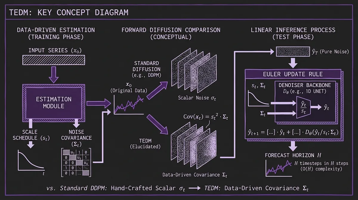
EDM's key contribution is separating the diffusion design into three cleanly independent axes: the noise schedule σt (how much noise is added at each diffusion step), the scale schedule st (how input magnitudes are normalized), and the preconditioning functions that ensure the network Fθ always sees unit-variance inputs regardless of noise level. The preconditioning is analytical — cskip, cin, cout are derived as closed-form functions of σt — so training is stable by construction.

The ablation in TEDM quantifies the benefit directly. Replacing iDDPM+DDIM with vanilla EDM (image-style, applied to time series without modification) already reduces MSE by 40% on ETTm2. TEDM's further modifications then add another 50% on top. The EDM baseline outperforms DDPM not because its backbone is different, but because the design space was elucidated correctly.

#Two Core Innovations

#Data-Driven Noise and Scale Schedules

TEDM's most important contribution is replacing hand-crafted schedules with schedules estimated directly from the input series.

The insight comes from the underlying Itô process that connects the diffusion trajectory to the observed data. At any diffusion step t, the conditional mean and covariance of the noised signal relate to the original data as:

E(xt) = st · E(x0)
Cov(xt) = s²t · Σt

These relationships mean both schedules can be estimated empirically from the data itself. TEDM implements two variants: cumulative estimation, which tracks running means and covariances from the start of the series, and sliding window estimation, which uses a rolling window to capture local non-stationarity. The better-performing variant (chosen per dataset on validation MSE) is used.

The practical effect is that the scalar σt of standard diffusion becomes a covariance matrix Σt, where each feature at each time step gets a noise level calibrated to its actual variance in the data. Heterogeneous multivariate series — where one column might be electricity consumption in megawatts and another is temperature in Celsius — receive appropriately scaled noise without manual normalization decisions.

The ablation results show this is the dominant source of TEDM's gains. On Exchange-Rate, data-driven Σt alone produces a 75% MSE reduction versus applying EDM with image-style schedules.

#Linear Inference Complexity

Standard diffusion-based forecasting incurs O(S × H) cost: S denoising steps for each of the H forecast horizon steps. For long horizons and many denoising steps, this becomes expensive quickly. Sundial addressed this with flow matching (fewer steps needed). TEDM takes a structurally different approach.

Because TEDM's backward ODE is formulated so that diffusion time and physical time coincide, each step of the inference rule advances the forecast window by exactly one timestep. Starting from the historical context, one network evaluation produces the next step; H evaluations produce the full horizon. The formula is a single Euler update per step:

ŷ_{t+1} = [I − log(st/st−1) · I] · ŷt
           + st · log(Σt) · Σ^{−1/2}_{t−1} · Dθ(ŷt/st; Σt)

This requires the diagonal approximation of Σt (full matrix operations for large feature sets would be prohibitive), and it holds exactly when Σt and its time derivative commute — a condition satisfied by systems where the relative relationships between features are stable even as overall noise intensity changes.

The efficiency numbers confirm this works: TEDM trains at 0.004 seconds per batch and uses ~21 MB of memory on ETTm2, compared to 0.022 s/0.759 GB for TimeDiff and 0.098 s/3.1 GB for DiffusionTS, while achieving meaningfully better MSE than both.

#Architecture

Unlike large pretrained TSFMs, TEDM is a family of lightweight architectures wrapped by the EDM preconditioning scheme. The paper evaluates five backbone designs for the denoiser network:

LinearNet — a single fully-connected layer applied along the temporal dimension. No recurrence, no attention. Remarkably competitive on several datasets, suggesting the preconditioning and schedule design do more work than the backbone capacity.

UNet — the primary architecture and best performer overall. Adapts the ADM architecture to 1D sequential data, with alias-free resampling, rotary position embeddings (RoPE), and 1D convolutional residual blocks with optional self-attention at selected scales.

AttnNet variants — single or stacked cross-attention layers attending from the noised input to the conditioning context, with varying degrees of noise-level conditioning.

ConvLSTMNet — 1D convolution followed by a bidirectional LSTM with noise-level embedding.

The model is conditioned on historical context through a strided backward window (kctx timesteps back), though the ablation reveals this conditioning is sometimes counterproductive — on some datasets, kctx=0 (no explicit historical conditioning) yields the best results. This is counterintuitive but consistent with the linear-inference framing: if the Euler update correctly propagates information through the series, an additional conditioning mechanism may introduce redundant or conflicting signal.

#Benchmark Results

TEDM is evaluated on eight standard datasets at H=96, compared against diffusion-based baselines and deterministic SotA.

#Where It Wins

Against diffusion baselines, TEDM achieves the best MSE on ETTh2, ETTm2, and Exchange-Rate. Against all methods including deterministic models (iTransformer, PatchTST, DLinear), TEDM is first on ETTh2 (0.214 vs. iTransformer's 0.297), ETTm2 (0.135 vs. 0.180), Exchange-Rate (0.069 vs. 0.086), and Stock (0.056 vs. 0.342 for iTransformer — a large gap).

The efficiency advantage is consistent regardless of accuracy ranking: TEDM uses the least memory and has the fastest training time of any diffusion method in the comparison set.

#Where It Struggles

ETTh1 is TEDM's clearest failure case. The dataset contains large-amplitude sudden changes that violate the smooth-flow assumption underlying the Itô process formulation. TEDM scores MSE 0.595 there — worse than all other diffusion methods and well behind iTransformer (0.386).

Solar-Energy (137 features) reveals the diagonal approximation's limits. At high feature dimension, assuming a diagonal covariance matrix becomes increasingly unrealistic, and TEDM scores MSE 1.061 against iTransformer's 0.203. Full matrix operations at this dimension would be computationally prohibitive, so the approximation is a practical necessity that carries a real accuracy cost.

#Model Comparison Summary

Method	ETTh2 MSE	ETTm2 MSE	Exchange MSE	Training (s/batch)	Memory (MB)
TEDM	0.214	0.135	0.069	0.004	21.3
ARMD	0.311	0.181	0.093	0.009	20.7
NsDiff	0.460	0.250	0.146	0.107	2,682
TimeDiff	0.364	0.209	0.208	0.022	759
iTransformer	0.297	0.180	0.086	—	—

#The Calibration Gap

TEDM's probabilistic results tell a more complicated story. When uncertainty is measured via CRPS — the standard metric for distributional forecast quality that we discuss in our prediction intervals deep-dive — TEDM's SDE-based sampling underperforms: 0.589 on ETTh2 versus NsDiff's 0.349 and TimeDiff's 0.380.

The authors are candid about this. The diagonal covariance approximation used for computational tractability does not accurately represent the correlated uncertainty structure in the full Σt matrix. Stochastic sampling from this approximated distribution produces intervals that are geometrically wrong, even when the mean forecast is excellent.

There is a more promising path: TEDM introduces a novel quantile-sampling procedure that extracts prediction intervals from the deterministic ODE rather than from stochastic sampling. Early results are strong — CRPS 0.294 on ETTh2 versus NsDiff's 0.349 — but the method's full theoretical development is deferred to future work. If that work lands, TEDM could become competitive on probabilistic metrics without the SDE sampling step.

This is an honest limitation to track. A model that wins on MSE but loses on CRPS is useful for point-forecast applications but not for risk-sensitive ones. The ODE quantile path is the one to watch.

#What TEDM Is and Isn't

It is worth being clear about where TEDM sits relative to the broader TSFM landscape. It is not a foundation model — it trains from scratch on each dataset, without pretraining on large corpora. It requires no GPU for training beyond what you already have (21 MB training memory is accessible on nearly any modern hardware). It is not zero-shot — you need labeled training data.

What it is: a rigorous application of diffusion model design principles to time series, yielding a lightweight model that achieves competitive or state-of-the-art MSE on several standard benchmarks while being faster and cheaper to train than any other diffusion-based forecaster. If you have a specific dataset, labeled training data, and care about accuracy efficiency tradeoffs more than zero-shot transfer, TEDM is a credible choice.

The contrast with Aurora — the other major diffusion-adjacent ICLR 2026 time series paper — is instructive. Aurora is a 0.4B parameter pretrained foundation model for zero-shot cross-domain inference. TEDM is a 1D UNet trained in hours on commodity hardware. Both use EDM-derived mathematics. They serve fundamentally different use cases, and neither makes the other obsolete.

#Why EDM for Time Series Matters Beyond TEDM

The deeper contribution here is the framework, not the numbers. Prior diffusion models for time series — TimeGrad, CSDI, TSDiff, NsDiff — each introduced problem-specific modifications to DDPM without reasoning about the underlying design choices. TEDM shows that applying EDM's design-space analysis to time series yields a principled path toward better models: identify the assumptions that don't hold (scalar schedules, isotropic noise, image-domain preconditioning), replace them with time-series-appropriate alternatives, and validate each substitution with ablation.

That methodology is reusable. Future work that extends TEDM to handle long-memory processes, full covariance structure for high-dimensional data, or integrates learned period structure (as Aurora does with its FFT image branch) would have a clean foundation to build on.

The paper's strongest claim — that EDM's modular design space translates directly to time series — is confirmed by the ablation. iDDPM → EDM → TEDM is a monotonic improvement across every tested dataset, which is what you expect when each step replaces an empirical heuristic with a principled alternative.