No Adjacency Matrix Required: TSFMs as Strong Baselines in Transportation Forecasting
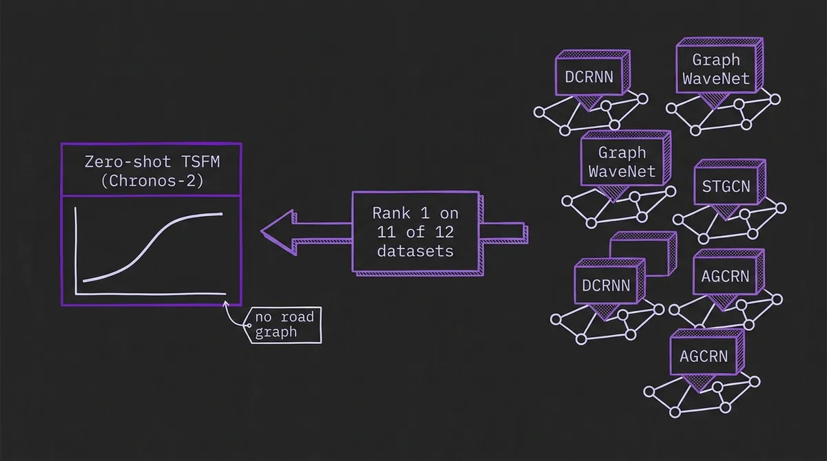
A new large-scale benchmark runs a zero-shot time series foundation model against the specialized graph neural networks that have owned traffic forecasting for years. Across ten transportation datasets, the foundation model ranks first on eleven of twelve metric groups, without ever seeing the road graph.
Transportation forecasting has been one of the most graph-shaped problems in machine learning. For years the leaderboards on datasets like METR-LA and PEMS-BAY have been owned by spatio-temporal graph neural networks: DCRNN, Graph WaveNet, STGCN, AGCRN, and a long tail of successors. The shared assumption is that to predict traffic you must encode the road network as an adjacency matrix and diffuse information along it. The structure is the point.
A new benchmark from Javier Yanes-Pulido and Filipe Rodrigues, Time Series Foundation Models as Strong Baselines in Transportation Forecasting, tests that assumption directly. The authors take a single time series foundation model, run it zero-shot with no task-specific training, and put it up against the full catalog of specialized architectures across ten real transportation datasets. The foundation model is Chronos-2, which TSFM.ai hosts. The result is the kind of finding that should reframe how the field sets its baselines: the model that never saw the road graph ranks first on eleven of twelve metric groups.
#What the Benchmark Actually Covers
This is not a single-dataset result dressed up as a trend. The study spans ten datasets across four distinct transportation modalities:
| Dataset | Domain | What is forecast |
|---|---|---|
| PeMSD7(M) | California highways | Traffic speed |
| PeMSD4 | California highways | Traffic volume |
| METR-LA | Los Angeles | Traffic speed |
| PEMS-BAY | SF Bay Area | Traffic speed |
| Seattle Loop | Seattle | Traffic speed |
| Urban1 | South Korea | Urban traffic speed |
| SZ-taxi | Shenzhen | Taxi-derived speed |
| NYC Citi Bike | New York | Bike-sharing demand |
| NYC Bike Flow | New York | Bike in/out flow |
| UrbanEV | Shenzhen | EV charging occupancy, sessions, volume |
The horizons range from a single 5-minute step on Seattle Loop to 12 hours on UrbanEV, covering the short-horizon nowcasting regime where graph models usually shine and the longer-horizon regime where they usually struggle. The comparison set is the real competition, not a strawman: classical baselines (ARIMA, VAR, historical average, XGBoost, SVR) alongside more than twenty specialized deep learning models including DCRNN, Graph WaveNet, STGCN, ASTGCN, AGCRN, STGODE, STG-NCDE, and T-GCN.
#The Headline Result
Across the twelve metric groups the authors tabulate, Chronos-2 ranks first on eleven. The only exception is METR-LA, where it lands third and slightly trails the historical-average baseline by about 12.6% MAE, which the authors attribute to dataset-specific dynamics rather than a systematic weakness.
The margins on its strong datasets are not marginal. Against the historical-average baseline, Chronos-2 improves MAE by roughly 46.6% on SZ-taxi and by about 70.5% on UrbanEV charging occupancy. These are gaps large enough that they are not explained by hyperparameter luck, and they hold against the specialized architectures, not just the classical baselines.
Two things make this more than a leaderboard curiosity.
First, it is fully zero-shot. Every specialized model in the comparison was trained on the target dataset, with its spatial structure, its sensor layout, and its traffic regime baked into the weights. Chronos-2 was handed the histories and asked to forecast cold. The DCRNN-lineage models get to learn the map. The foundation model does not, and still wins most of the time.
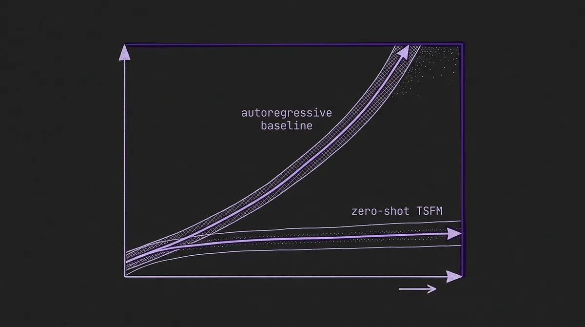
Second, the advantage grows with horizon. The paper notes that Chronos-2's accuracy stays stable as the forecast horizon extends, in contrast to the autoregressive error accumulation that degrades many traditional approaches. Long-horizon traffic and demand forecasting is exactly where operational value concentrates, because that is the regime in which dispatch, rebalancing, and charging decisions are actually made.
#Why a Graph-Blind Model Competes on a Graph Problem
The interesting question is not that Chronos-2 wins, but how a model with no adjacency matrix competes with models built entirely around one.
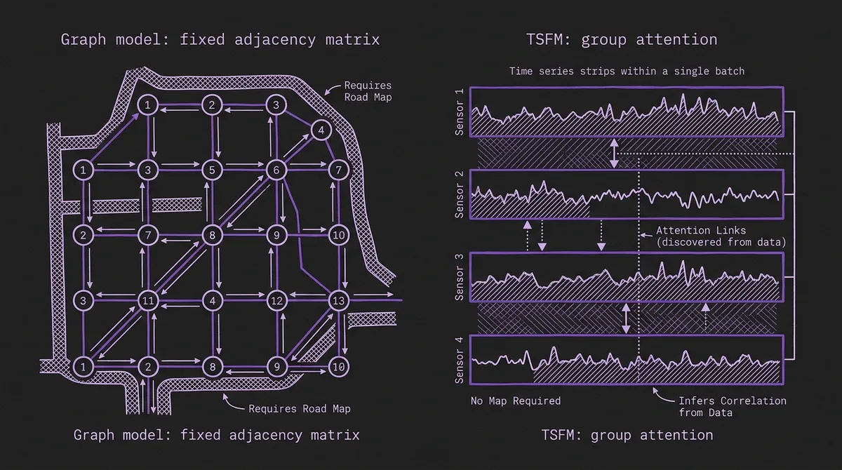
The authors point to Chronos-2's group attention mechanism. Rather than encoding spatial relationships through a fixed graph, the model attends across the series presented together in a batch, and in doing so it implicitly shares information between correlated locations. A loop detector on a congested corridor and its upstream neighbor produce statistically coupled series; group attention can exploit that coupling without anyone telling the model the two sensors are adjacent. This is the same multivariate capability we covered in the Chronos-2 universal forecasting writeup and in our survey of multivariate state of the art, applied here to a domain that assumed it needed explicit topology.
This matters because the fixed-adjacency assumption is also a fixed cost. A graph model is tied to the sensor layout it was trained on. Add a corridor, re-mesh a city, deploy in a new metro, and you are retraining. A foundation model that infers correlation from the data at inference time sidesteps that entire maintenance burden, which is the operational argument we made in the true cost of building and maintaining forecast pipelines. The benchmark is, in effect, an empirical measurement of how much that explicit structure was really buying.
#The Uncertainty Story, Told Honestly
Point accuracy is only half of what transportation operators need. Bike rebalancing, taxi positioning, and EV charging provisioning are all decisions under uncertainty, so calibrated intervals matter as much as the median forecast. Here the benchmark gives a more nuanced picture, and it is worth reading honestly rather than selectively.
Chronos-2 produces native probabilistic output, so prediction intervals come for free without a separate quantile model. On UrbanEV charging occupancy, its empirical coverage at the 80% nominal level is 78.24%, which is close to target and genuinely useful. But across the full set, coverage ranges from about 63% to 80%, and the model is meaningfully under-covered on SZ-taxi (63.42%) and NYC Citi Bike (63.87%). The authors tie this to datasets with frequent zero observations: sparse, bursty, zero-inflated demand is hard to wrap a calibrated interval around, and a zero-shot model has no chance to learn the dataset's specific tail behavior.
The practical reading is the same one we have given for other domains. Use the native intervals as a strong starting point, then apply conformal recalibration on a holdout window when coverage matters operationally. The distinction between raw and recalibrated intervals, and why it matters for downstream decisions, is the subject of our point forecasts versus prediction intervals post. None of this undermines the headline; it sharpens it. The model is a strong out-of-the-box forecaster whose intervals are good on dense series and need a calibration pass on sparse ones.
#How This Fits the Broader Pattern
Transportation now joins a growing list of domains where a general-purpose foundation model, used zero-shot, matches or beats the specialized stack that domain spent years building. We have documented the same shape in telecom and network traffic, in energy demand, and in production retail demand. Each domain assumed its structure was special. In each case the foundation model captured enough of that structure implicitly to be competitive, and arrived with zero-shot deployment and native uncertainty as a bonus.
The authors are careful, and so should we be: the claim is not that graph neural networks are obsolete. On a dataset like METR-LA, a well-tuned specialized model still has an edge, and for a fixed, stable, heavily instrumented network where you can amortize training cost, a purpose-built model may remain the right call. The claim is narrower and more durable: a zero-shot TSFM is now a strong default baseline that any new transportation forecasting method should have to beat. Publishing a graph model in 2026 without comparing against a hosted foundation model is leaving the most informative baseline off the table.
For practitioners, the takeaway is concrete. If you are standing up traffic, bike-share, taxi, or EV-charging forecasting, the fastest credible first system is no longer a multi-week graph-model training effort. It is a zero-shot foundation model you can evaluate on your own series this afternoon, with a calibration pass where coverage matters and a model-routing layer if different parts of the network behave differently enough to warrant it. You can try Chronos-2 against your own transportation series directly in the TSFM.ai playground. The graph models had a remarkable run. The benchmark says the baseline has moved.
Primary sources: Time Series Foundation Models as Strong Baselines in Transportation Forecasting (arXiv:2602.24238), Chronos-2 (arXiv:2510.15821), DCRNN, the origin of the METR-LA and PEMS-BAY benchmarks (arXiv:1707.01926). Benchmark context from our GIFT-Eval deep dive.