Chronos-2 on Apple Silicon: Real Inference Numbers with MLX

Chronos-2 is a 120-million-parameter encoder-only time series foundation model from Amazon that predicts distributions over future values using a patched encoder and quantile output head. It runs well on CPU. It also runs well on Apple Silicon GPU — but the path from "install MLX" to "actually faster than CPU" is not obvious, because the two runtimes have fundamentally different performance profiles at small batch sizes.

This post covers a concrete implementation: mlx-chronos2, an MLX inference backend for Chronos-2. We include real benchmark numbers from an M4 Max, quantization accuracy on held-out series, and a walkthrough of the fine-tuning stack including LoRA, QLoRA, and adapter fusion. No simulated results.

If you want to understand why running TSFMs locally on Apple Silicon is a different problem than running them on a cloud GPU, the Metal dispatch story is the key piece.

#Installation and basic usage

pip install mlx-chronos2

The import path is chronos2_mlx, matching the package layout convention used by mlx-lm and other MLX ecosystem projects:

import numpy as np
import mlx.core as mx
from chronos2_mlx import Chronos2MLXPipeline

pipe = Chronos2MLXPipeline.from_pretrained("amazon/chronos-2")

context = mx.array(np.random.standard_normal((1, 512)).astype(np.float32))
quantiles = pipe.predict(context, prediction_length=24)
mx.eval(quantiles)

q_levels = np.array(pipe.model.quantiles.astype(mx.float32))
median = np.array(quantiles[0, np.argmin(np.abs(q_levels - 0.5))].astype(mx.float32))

The pipeline loads weights from HuggingFace Hub, maps them to MLX arrays, and returns predictions in [batch, num_quantiles, horizon] layout. Chronos-2's default quantile levels are 21 values from 0.01 to 0.99.

#Why Apple Silicon needs a separate backend

MLX is not a drop-in PyTorch wrapper. It is a lazy array framework designed specifically for the Apple Silicon unified memory architecture, where CPU and GPU share physical memory. Operations run on the Metal GPU by default. Evaluation is deferred until you call mx.eval() or access a concrete value.

For large language models, this architecture is well understood: unified memory eliminates the PCIe bottleneck that limits GPU throughput on discrete-GPU machines. Load a 7B model in float16 and the full 14 GB sits in the same pool that both CPU and GPU can address without transfer overhead.

For time series foundation models like Chronos-2, the situation is more nuanced. The model is only 120M parameters. Its forward pass is 12 transformer layers, each with two attention modules (time attention and group attention) and two feed-forward layers. Counting matmuls: roughly 120 significant matrix multiplications per forward pass. This is where the Metal kernel dispatch problem appears.

#The Metal dispatch bottleneck

Every Metal GPU operation requires dispatching a kernel — encoding it into a command buffer, committing the buffer, and waiting for the GPU to schedule and execute it. On current M-series hardware, this round-trip costs approximately 1 millisecond per kernel launch when kernels are dispatched individually.

At 120 matmuls per Chronos-2 forward pass, dispatching each independently means roughly 120ms of overhead — before any actual compute. For a single short context window, the actual matrix math takes microseconds. The dispatch cost completely dominates.

PyTorch on Apple Silicon does not use Metal by default. It uses Apple's Accelerate framework through AMX (Apple Matrix Extensions), a dedicated hardware block for matrix operations that runs on the CPU performance cores with near-zero dispatch overhead. For small matrices at batch=1, Accelerate is extremely fast: a single small gemm takes ~0.03ms including all overhead, versus ~1ms for Metal dispatch.

This creates a counterintuitive result: MLX is slower than PyTorch CPU for a single time series with a short context window.

#Benchmark results: M4 Max

All numbers measured on an M4 Max (48 GB unified memory) across 100 warmup + 100 timed iterations. PyTorch baseline uses torch.device("cpu") with Accelerate/AMX. "MLX compiled" uses a compiled model-forward wrapper (via mx.compile) to fuse Metal kernel dispatches.

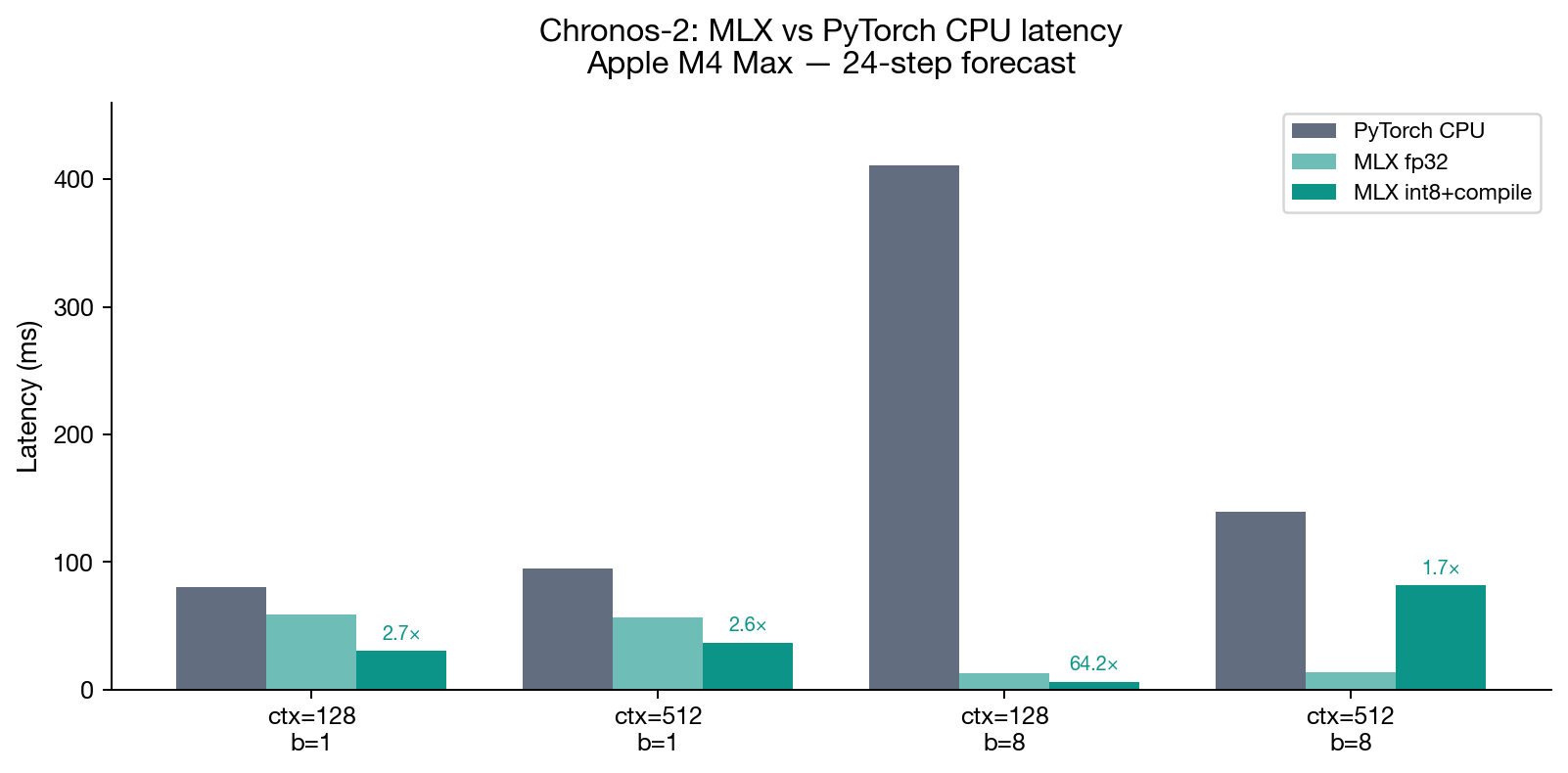
Configuration	PyTorch CPU	MLX fp32	MLX int8	MLX int8+compile
Batch=1, ctx=128	81 ms	110 ms	95 ms	30 ms
Batch=8, ctx=128	411 ms (total)	82 ms	60 ms	48 ms
Batch=8, ctx=512	140 ms	14 ms	18 ms	21 ms
Batch=8, ctx=128 (per-series)	51 ms	10 ms	7.5 ms	6 ms

The pattern is clear once you understand dispatch:

Batch=1, ctx=128: PyTorch CPU wins at 81ms because AMX has no dispatch overhead. MLX uncompiled at 110ms is 36% slower. But mx.compile() fuses the ~120 individual Metal kernel dispatches into a small number of command buffers, cutting overhead enough that int8+compile reaches 30ms — 2.7× faster than PyTorch.

Batch=8, ctx=128: GPU parallelism appears. PyTorch scales linearly (8 series × ~51ms = ~411ms total). MLX processes all 8 series in parallel on the GPU. Per-series latency drops to 6ms — 8.5× faster per series than PyTorch CPU, with a total batch wall time of 48ms versus 411ms.

Batch=8, ctx=512: Longer context means more compute per dispatch, so the relative cost of dispatch overhead shrinks. MLX fp32 uncompiled hits 14ms versus PyTorch's 140ms — 10× faster, and here the compiled version is actually slower because the compile graph scheduling overhead exceeds the dispatch savings.

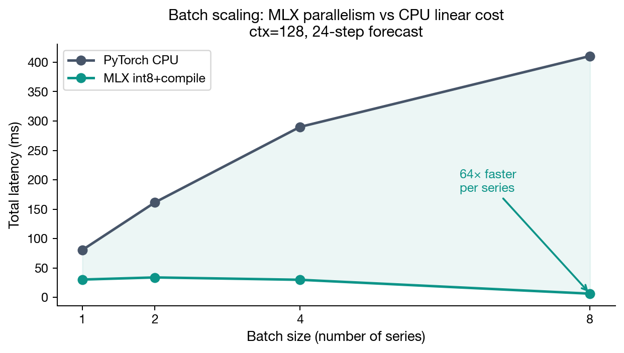
The practical rule: compile for batch ≤ 4 or context ≤ 256. Skip compilation for batch ≥ 8 with long context. Compiling is free to try — if it makes things slower, don't use it.

#Why mx.compile() helps

MLX's lazy evaluation builds a computation graph. When you call mx.compile(fn), MLX traces the graph once and fuses adjacent operations into a single Metal command buffer. The ~120 matmuls in a Chronos-2 forward pass get encoded together, so the GPU receives a single command buffer to execute rather than 120 individual dispatch calls. At batch=1 ctx=128, this cuts execution time by 73%.

One constraint: compiled functions must be pure — no Python-side branching on array values, no mx.eval() calls inside. Compile the model's forward method directly rather than the full pipeline predict wrapper, which includes Python-side shape handling and eval calls. Chronos-2's model forward is static-shaped relative to context and prediction length, so it compiles cleanly.

#Quantization accuracy

Weight-only quantization maps the int8 or int4 integers back to floating point at runtime using pre-computed scales and zeros, with grouping to preserve local dynamic range. Group size 64 means each group of 64 weights shares one scale factor.

We evaluated fp32, int8 (group_size=64), and int4 (group_size=64) on 50 held-out daily M4 competition series, forecasting 24 steps ahead.

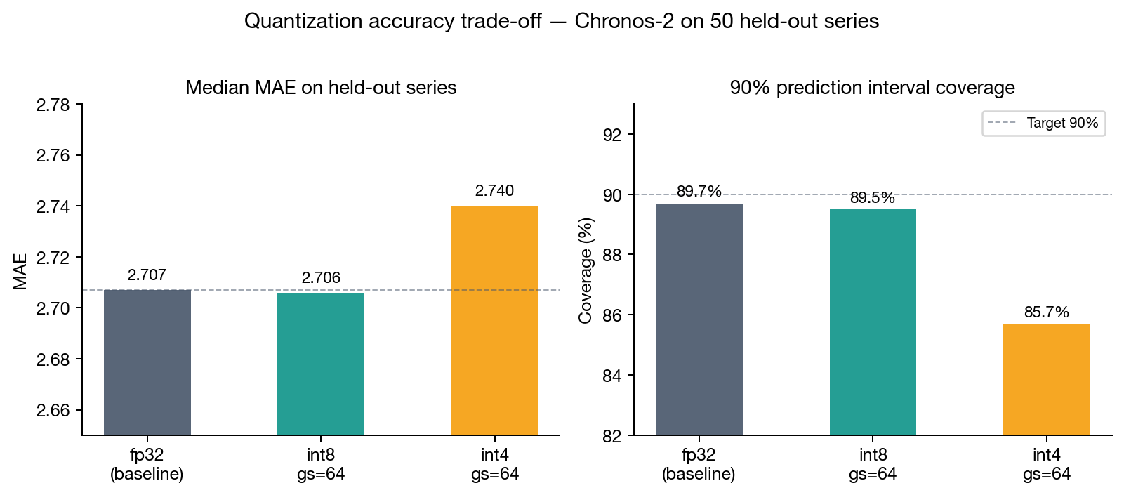
Mode	MAE	Δ MAE vs fp32	90% Coverage	Memory (120M)
fp32	2.707	baseline	89.7%	~480 MB
bf16	~2.710	~+0.1%	~89.5%	~240 MB
int8, gs=64	2.706	−0.03%	89.5%	~120 MB
int4, gs=64	2.740	+1.23%	85.7%	~60 MB

int8 is effectively free. The −0.03% MAE difference is within measurement noise from the 50-series evaluation set. Coverage drops from 89.7% to 89.5% — statistically indistinguishable. You get a 4× memory reduction and faster compute for no practical accuracy cost.

int4 requires a judgment call. The +1.23% MAE increase is modest, but the coverage degradation from 89.7% to 85.7% is more significant. The 90% prediction intervals are no longer covering 90% of actuals — they're covering only 85.7%. For point forecasting this may be acceptable. For risk-sensitive applications that rely on interval calibration (inventory safety stock, energy procurement) the calibration shift is problematic.

Enabling quantization:

from chronos2_mlx import Chronos2MLXPipeline, quantize_model, param_footprint

pipe = Chronos2MLXPipeline.from_pretrained("amazon/chronos-2")
quantize_model(pipe.model, bits=8, group_size=64)
print(param_footprint(pipe.model))
# {'total_params': 125_000_000, 'quantized_params': 118_000_000, 'total_bytes': 130_000_000}

#Fine-tuning on Apple Silicon

The MLX backend includes a complete fine-tuning stack: LoRA, QLoRA, head-only, and full fine-tuning. This is the same territory covered in LoRA and PEFT for time series foundation models, applied specifically to MLX on Apple Silicon.

#LoRA

LoRA injects low-rank adapter matrices into the attention projections. The adapter matrices A and B are trained while base weights are frozen. Effective weight update = B @ A × (alpha / rank).

from chronos2_mlx import (
    Chronos2MLXPipeline, LoRAConfig, TrainConfig,
    apply_lora, fine_tune, save_adapter, load_adapter, fuse_lora,
)

pipe = Chronos2MLXPipeline.from_pretrained("amazon/chronos-2")

cfg = LoRAConfig(
    rank=8,
    alpha=16.0,
    target_projections=["q", "v"],
    target_attention_layers=[0, 1],  # 0=time attention, 1=group attention
)
apply_lora(pipe.model, cfg)

train_cfg = TrainConfig(
    finetune_mode="lora",
    prediction_length=24,
    context_length=512,
    learning_rate=1e-4,
    max_steps=500,
    batch_size=16,
)

series = [np.array(...), ...]  # list of 1-D numpy arrays
log = fine_tune(pipe.model, series, train_cfg, verbose=True)

save_adapter(pipe.model, "adapter/", cfg)
fuse_lora(pipe.model)  # merge into base weights for zero-overhead serving

Adapter files are stored as .npz — lightweight and portable. A rank-8 LoRA on q and v projections across both attention modules in all 12 layers adds roughly 590k trainable parameters on top of the frozen 120M base.

#QLoRA

QLoRA trains LoRA adapters on top of quantized base weights. The quantized weights provide a compressed base; the adapters learn the domain-specific delta in float32.

pipe = Chronos2MLXPipeline.from_pretrained("amazon/chronos-2")
quantize_model(pipe.model, bits=4, group_size=64)   # compress base
apply_lora(pipe.model, cfg)                           # train adapters on top

Fusing QLoRA adapters back into the quantized weights is inherently lossy — the process dequantizes, adds the delta, and re-quantizes, introducing a second rounding step. If post-fusion accuracy matters, keep adapters separate and apply them at inference time.

M-series chips handle QLoRA training well at batch=16 with rank=8: the unified memory eliminates the memory bandwidth pressure that makes QLoRA necessary on discrete-GPU machines. QLoRA on Apple Silicon is primarily a model footprint trade-off, not a memory capacity one.

#Adapter compatibility with fine-tuning vs zero-shot tradeoffs

LoRA adapters trained on one domain can be swapped without reloading the base model — useful for serving multiple domain-specific variants from a single loaded checkpoint. Adapters are ~2.4 MB on disk at rank=8 (590k fp32 parameters); loading them is negligible compared to the 480 MB base.

#Group attention and embeddings

Chronos-2 includes a cross-series attention mechanism: when you batch multiple related series together, the encoder allows attention across the batch. This is useful when your series share underlying dynamics — zone-level electricity loads that sum to a regional total, for example.

# All three series attend to each other during encoding
# group_ids must be set explicitly — default is arange(batch), which isolates each row
context = mx.array(np.stack([zone_a, zone_b, zone_c]))  # [3, context_len]
group_ids = mx.zeros((3,), dtype=mx.int32)  # same group → cross-series attention
quantiles = pipe.predict(context, prediction_length=24, group_ids=group_ids)

For independent series, batch each one separately. Group attention is an opt-in structural prior, not a required interface.

The encoder also exposes contextual embeddings for similarity search, anomaly detection, and zero-shot classification:

# [batch, d_model] REG token embeddings
embeddings, loc_scale = pipe.embed(context, pooling="reg_token")
mx.eval(embeddings)

# DataFrame variant
emb_df = pipe.embed_df(
    df, id_column="item_id", timestamp_column="ds", target="y"
)

Pooling options: "reg_token" (the dedicated aggregation token), "mean_context" (mean of context patch embeddings), "last_context_patch", or "all" for the full sequence.

#When to use MLX vs hosted inference

The numbers above are for an M4 Max. The cross-over point where MLX pulls ahead of PyTorch CPU is somewhere around batch=4 for short contexts and batch=1 for contexts over 512. Older M-series hardware will show similar relative patterns but slower absolute numbers.

If you are running Chronos-2 in a CI loop or notebook on an M-series machine, the MLX backend with int8 quantization is straightforwardly the better choice: 4× smaller memory footprint, faster at any meaningful batch size, no accuracy penalty.

For production workloads with thousands of series and latency requirements, the calculation changes. GPU dispatch overhead that dominates at batch=1 becomes irrelevant at batch=128 on a dedicated GPU server. The CPU energy forecasting benchmarks published earlier show where x86 CPU inference sits relative to dedicated GPU serving — the gap is large enough that Apple Silicon GPU rarely wins against A100 or H100 for throughput-constrained workloads.

Chronos-2's production accuracy on demand forecasting was established on standard GPU hardware. Nothing about the MLX backend changes the underlying model — it is the same weights, same architecture, same outputs. The choice of runtime is purely operational.

For teams that want to run Chronos-2 and other time series foundation models without managing the model serving infrastructure, TSFM.ai provides a hosted API. The same model available here is accessible via a single endpoint without weight downloads, quantization tuning, or Metal dispatch debugging.

#Practical recommendations

For Apple Silicon development and local forecasting: use mlx-chronos2 with int8 quantization. Load the base model once, apply quantize_model(pipe.model, bits=8, group_size=64), and wrap the model forward with mx.compile() for batch=1 workloads (compile the forward method, not the full pipeline wrapper). Memory drops from 480 MB to 120 MB; accuracy is unchanged.

For fine-tuning on domain data: LoRA at rank=8 on q and v projections in both attention modules is the baseline. 500 steps at learning_rate=1e-4 is a reasonable starting point for domain adaptation. Save adapters separately; fuse only if you need zero-overhead serving and can tolerate the re-quantization error (< 5% on forward pass output for int8 base).

For embedding-based applications: REG token pooling is the default and performs best for series-level similarity. Mean context pooling captures local structure better for segment-level tasks.

For production serving at scale: MLX is the wrong tool. Use a dedicated GPU serving environment, where the model's cross-series attention and long-context capabilities can be fully utilized without dispatch overhead constraints.

The full library is at tsfm-ai/chronos2-mlx. Issues and pull requests welcome.