QuitoBench: What a Billion-Scale Benchmark Reveals About When to Use Foundation Models

Most time series benchmarks ask the wrong question. They organize datasets by application domain — electricity, traffic, weather, healthcare — and compute aggregate metrics across those buckets. The underlying assumption is that domain is a useful proxy for forecasting difficulty. It often is not. Two traffic series can differ more in predictability than a traffic series and an electricity series with similar statistical structure. And because different model families have different strengths across statistical regime types, domain-aggregated metrics can obscure the signals that actually matter for deployment decisions.

QuitoBench, a new benchmark from Ant Group published in March 2026, takes a different approach. Instead of grouping series by what they represent, it groups them by how they behave — specifically, by the combination of trend strength, seasonality strength, and forecastability of each series. The result is an eight-cell TSF regime taxonomy that reveals patterns that are hard to see in prior evaluations: a context-length crossover between deep learning and foundation models, a dominant effect of forecastability on difficulty, and concrete model-selection rules for practitioners.

The benchmark is built on Quito, a billion-scale corpus of application traffic telemetry from Alipay's production platform. The authors position it as a cleaner evaluation substrate than heterogeneous public benchmark assemblies because it is single-provenance, uniformly long, and constructed to support regime-balanced evaluation at multiple context lengths.

#The Problem With Domain-Based Evaluation

The standard critique of existing benchmarks is well known — we have covered it in depth previously. But QuitoBench's authors quantify a specific structural weakness that is worth highlighting: existing benchmarks can be heavily imbalanced by regime.

The paper reports that when GIFT-Eval's series are re-labeled by TSF regime rather than domain label, 50.7% of all series fall into a single regime cell. It also reports that the Timer benchmark suite — ETT, ECL, Traffic, Weather, PEMS — concentrates 65.8% of series in the high-seasonality, high-forecastability regime. Aggregate metrics computed over those distributions are dominated by whichever regime happens to be most prevalent. A model that excels at strongly seasonal, highly forecastable series can therefore rank first on these benchmarks while telling you less about performance on harder, lower-forecastability workloads.

The imbalance also limits what you can measure about context length. Context length is one of the most consequential configuration choices in TSFM deployment, yet the paper notes that 50% of GIFT-Eval series contain fewer than 200 time points, which sharply restricts evaluation at longer history windows. You cannot observe a crossover you cannot measure.

QuitoBench's design directly addresses both issues. The benchmark distributes evaluation instances near-uniformly across all eight TSF regime cells (roughly 12% per cell), and all underlying series are uniformly long (5,900–15,300 time steps), enabling evaluation at context lengths up to L=1,024.

#The TSF Regime Framework

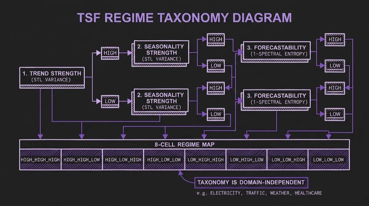
The regime taxonomy is built on three diagnostics, each computed per series and binarized at a threshold of τ=0.4:

Trend strength (T): The fraction of variance explained by the trend component of an STL decomposition. A high-trend series exhibits long-range drift; a low-trend series is mean-reverting or stationary.

Seasonality strength (S): The fraction of variance explained by the seasonal component of the STL decomposition. A high-seasonality series has regular, recurring periodic structure; a low-seasonality series does not.

Forecastability (F): Defined as F = 1 − H, where H is the normalized spectral entropy (Welch's method). A high-forecastability series has most of its power concentrated in a small number of spectral components; a low-forecastability series has more broadly distributed spectral energy.

Combining three binary diagnostics gives 2³ = 8 TSF regime cells, labeled by convention as TREND_SEASONALITY_FORECASTABILITY — for example, HIGH_LOW_LOW denotes a series with strong trend, no meaningful seasonality, and low forecastability.

This taxonomy is explicitly designed to be independent of domain. An electricity series and a web traffic series can share the same TSF regime. Two series from the same domain can sit in very different regime cells. The paper's central argument is that regime cell is often more informative than domain label for understanding difficulty and model behavior.

#The Quito Dataset

The benchmark is grounded in Quito, a single-provenance time series corpus collected from Alipay's production platform. Quito comprises two subsets:

• Quito-Min: 22,522 series at 10-minute granularity, covering approximately 6 weeks of workload data (~0.7 billion tokens)
• Quito-Hour: 12,544 series at hourly granularity, covering roughly two years of traffic (~1.0 billion tokens)

Together, the dataset contains 1.6 billion tokens across nine business verticals: finance, e-commerce, advertising, platform infrastructure, risk and compliance, and others from across Alipay's production stack.

Two design properties matter most for benchmark integrity:

Single provenance: All series originate from the same operational environment. That reduces overlap risk with public pretraining corpora and avoids mixing data sources with very different collection processes and artifacts.

Uniformly long series: Series span 5,904 steps (Quito-Min) and 15,356 steps (Quito-Hour). This enables rolling-window evaluation at context lengths of L = 96, 576, and 1,024 — far beyond what most public benchmarks can support — which makes the context-length crossover measurable.

#Finding 1: The Context-Length Crossover

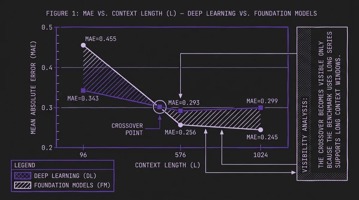
The headline result in QuitoBench is a crossover between deep learning and foundation models as context length increases:

Context Length (L)	FM MAE	DL MAE	Winner
96	0.455	0.343	Deep Learning (−24.6%)
576	0.256	0.293	Foundation (+14.8%)
1,024	0.245	0.299	Foundation (+22.0%)

At L=96, the best deep learning models (led by CrossFormer at ~1M parameters) beat the best foundation models (Chronos-2 at ~100M parameters) by 24.6%. At L=576, the direction reverses: foundation models are 14.8% better. At L=1,024, the foundation model advantage grows to 22.0%.

The paper does not present a mechanistic proof for why this crossover occurs, but the operational implication is still clear. Context length is not just a configuration choice driven by data availability or latency budget; in this benchmark it is also a model-selection signal. If you can provide L ≥ 576 steps of history, a foundation model is more likely to outperform a compact DL model. If you are constrained to L ≤ 96, the reverse is more likely to be true.

This finding complements prior work on context window effects in TSFMs and gives practitioners a concrete threshold to test rather than a purely qualitative recommendation.

#Finding 2: Forecastability Is the Dominant Difficulty Axis

The regime analysis reveals that forecastability — more than trend or seasonality in isolation — is the primary driver of forecasting difficulty:

TSF Regime	Mean MAE	Rank
HIGH_HIGH_HIGH	0.205	1 (easiest)
LOW_LOW_HIGH	0.220	2
LOW_HIGH_HIGH	0.299	3
LOW_HIGH_LOW	0.359	4
HIGH_LOW_HIGH	0.376	5
LOW_LOW_LOW	0.456	6
HIGH_HIGH_LOW	0.478	7
HIGH_LOW_LOW	0.749	8 (hardest)

The gap from easiest (HIGH_HIGH_HIGH, MAE 0.205) to hardest (HIGH_LOW_LOW, MAE 0.749) is 3.64×. For comparison, the paper reports a 1.32× gap for trend strength alone and a 1.51× gap for seasonality alone. Forecastability dominates both.

The hardest regime — HIGH_LOW_LOW, meaning high trend, low seasonality, low forecastability — is where every model struggles. Even CrossFormer, the best model overall, reaches MAE 0.600 in this regime. Statistical baselines fail badly (ES: MAE 1.061; SNaive: MAE 1.091), and even Chronos-2 reaches only 0.628. No evaluated model performs especially well here.

The forecastability metric (1 minus normalized spectral entropy) is computable from the training data before model selection. That creates an actionable preprocessing step: characterize your series by spectral entropy before choosing a model or setting accuracy expectations.

Foundation models are also more robust to low forecastability in this benchmark: the ratio of LOW to HIGH forecastability MAE is 1.74–1.75× for TSFMs versus 2.04–2.28× for deep learning models.

#Finding 3: Parameter Efficiency Versus Context-Length Regime

CrossFormer (~1M parameters) is dramatically smaller than the foundation models in the benchmark, which average about ~110M parameters. The aggregate parameter ratio is 59×, and on the overall leaderboard the DL category achieves slightly lower MAE than FM (0.279 vs. 0.314).

However, that aggregate summary masks the crossover. Disaggregated by context length, the picture is different:

Metric	Foundation Models	Deep Learning
Avg. Parameters	~110M	~1.9M
MAE at L=96	0.455	0.343 (DL −25%)
MAE at L≥576	0.250	0.296 (FM −15%)
Mean MAE overall	0.319	0.311 (DL −2%)

The 59× parameter-efficiency claim is therefore mostly a short-context story. At long context, foundation models earn their parameter budget. A practitioner deploying at L=96 can achieve equivalent or better accuracy with a much smaller model. A practitioner deploying at L=1,024 gets materially better accuracy from the larger pretrained model.

This has direct implications for model selection decisions. The question "is a foundation model worth the inference cost?" depends heavily on your context window.

#Finding 4: Data Scaling Dominates Model Scaling

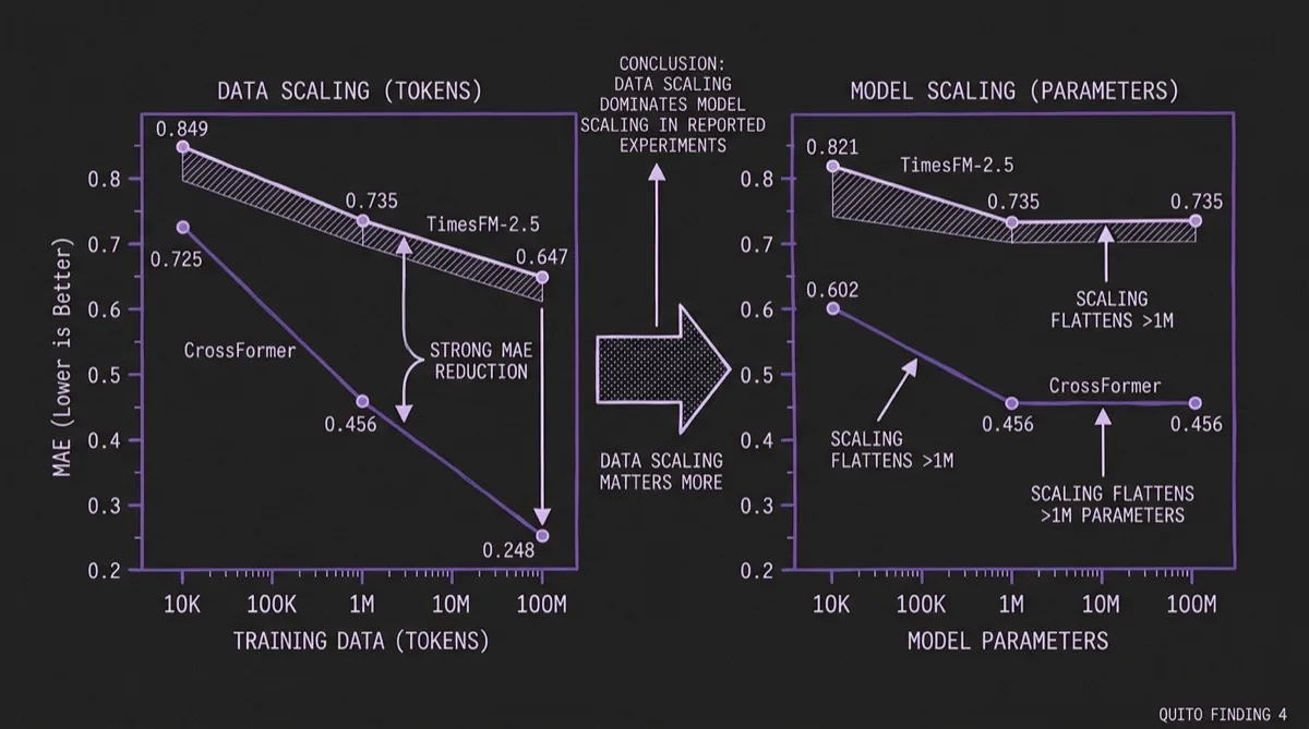
QuitoBench enables controlled data-scaling experiments because Quito is large enough to sub-sample at different training set sizes. The results challenge the assumption that model size is the primary lever:

Scale Dimension	Scale	CrossFormer MAE	TimesFM-2.5 MAE
Data (tokens)	10K	0.725	0.849
Data (tokens)	1M	0.456	0.735
Data (tokens)	100M	0.248	0.647
Model (params)	10K	0.602	0.821
Model (params)	1M	0.456	0.735
Model (params)	100M	0.456	0.735

Scaling from 10K to 100M training tokens produces a 66% MAE reduction for CrossFormer and a 24% reduction for TimesFM-2.5. Scaling model parameters over the same range produces no additional gain for CrossFormer beyond 1M parameters and similarly flattens for TimesFM-2.5 within the scales tested here.

That result is especially actionable for Timer-S1-style large-scale pretraining investments. For a fixed compute budget, increasing training data appears more valuable than simply increasing parameter count, at least up to roughly ~200M parameters and ~100M tokens in this study.

For teams considering fine-tuning a foundation model on domain data, the same logic applies: the first priority should usually be collecting more domain-specific training examples, not just selecting a larger base model.

#Regime-Specific Model Selection

The TSF regime analysis also surfaces a nuanced picture at the per-regime level. At the category level, FM models win 6 of 8 regime cells. But CrossFormer (the best DL model) beats Chronos-2 (the best FM) in 4 of 8 cells:

TSF Regime	CrossFormer MAE	Chronos-2 MAE	Winner
HIGH_HIGH_HIGH	0.165	0.163	FM
HIGH_HIGH_LOW	0.356	0.353	FM
HIGH_LOW_HIGH	0.180	0.349	DL (+38.4%)
HIGH_LOW_LOW	0.600	0.628	DL
LOW_HIGH_HIGH	0.199	0.197	FM
LOW_HIGH_LOW	0.239	0.235	FM
LOW_LOW_HIGH	0.154	0.207	DL (+17.7%)
LOW_LOW_LOW	0.370	0.397	DL

The practical pattern is that DL models win in all four low-seasonality cells, while foundation models win in all four high-seasonality cells. That makes seasonality strength a useful screening signal when deciding whether foundation models are likely to justify their extra size and inference cost.

This suggests that before deploying a foundation model, computing seasonality strength on a training sample is a fast way to decide whether you should benchmark a simpler DL baseline alongside it.

#Practical Takeaways for TSFM Practitioners

QuitoBench translates into a decision flow that can be applied before model selection:

Step 1: Compute your series' TSF profile. Run STL decomposition and spectral entropy on a sample of your training data. You need trend strength (T), seasonality strength (S), and forecastability (F = 1 − spectral entropy).

Step 2: Check forecastability first. If F is consistently low (< 0.4), every model family struggles more. Foundation models degrade less than DL models in this benchmark, but neither delivers strong accuracy on truly unpredictable series.

Step 3: Check your available context length. If you can provide L ≥ 576 steps of history, a foundation model (Chronos-2, TimesFM-2.5) is more likely to outperform a compact DL model. If you are constrained to L = 96, a well-trained compact DL model (CrossFormer-class) is more likely to match or beat a larger FM.

Step 4: Check seasonality. If your series lack strong seasonality (S < 0.4), DL baselines remain very competitive. In this benchmark, foundation model advantages concentrate in the high-seasonality cells.

Step 5: Prioritize data over model size. If you are considering fine-tuning, collecting 10–100× more domain-specific training data may produce larger gains than upgrading to a larger base model.

#Benchmarking Methodology Notes

The 232,200 evaluation instances are generated via dense rolling-window evaluation across:

• 3 context lengths: L = 96, 576, 1,024
• 3 forecast horizons: H = 48, 288, 512
• 2 variate modes: univariate (UV) and multivariate (MV)

The paper also reports cross-benchmark consistency with the Timer benchmark suite (Spearman ρ = 0.865, p < 0.01) and cross-metric consistency between MAE and MSE (mean Spearman ρ = 0.847 per configuration), supporting the claim that the benchmark's rankings are not purely artifacts of one metric choice.

The paper includes explicit comparisons to GIFT-Eval and FEV Bench to situate the findings within the existing evaluation landscape, and the code, data, and evaluation framework are open-sourced with data available on HuggingFace.

#Bottom Line

QuitoBench is a strong attempt to reframe time series benchmarking around statistical regime rather than domain label. Its core contribution is not a new model but a different way of organizing the evaluation question. By replacing domain buckets with TSF regimes and building on a billion-scale, single-provenance corpus, it surfaces model-selection patterns that are easier to act on in practice.

The context-length crossover alone — DL wins at L=96, TSFMs win at L≥576 — is a concrete operational rule. The forecastability result reframes how to think about difficulty. The data-scaling result pushes against the instinct to solve forecasting problems mainly by selecting larger models.

Foundation models are not uniformly better than compact DL models. In QuitoBench they are better in specific regimes — longer context, stronger seasonality, and moderate-to-high forecastability — and worse in others. Knowing which regime you are in is, with this benchmark, a more tractable problem than it was before.

---

Primary sources: QuitoBench paper (arXiv:2603.26017), QuitoBench project website, Quito dataset on HuggingFace, source code on GitHub.