TIME: Why Task-Centric Zero-Shot Evaluation Changes How We Compare TSFMs

Every major TSFM benchmark published before 2026 inherits the same structural problem: its datasets were already old when the benchmark launched. ETTh1, Electricity, Traffic, and Weather — the canonical long-sequence forecasting datasets — have been cycling through pretraining corpora and evaluation suites for years. GIFT-Eval addressed this by carefully selecting datasets unlikely to appear in pretraining corpora. FEV Bench made contamination tracking an explicit methodological requirement. But both still draw heavily from the same established archives, and both evaluate models using horizon settings defined by mechanical rules (fixed horizons, frequency-proportional lengths, or fixed split ratios) rather than the operational context that makes a forecasting task meaningful.

TIME (arXiv:2602.12147), from researchers at Nanyang Technological University, Tsinghua University, Monash University, and collaborating institutions, proposes a different starting point. Published in February 2026, it introduces a task-centric benchmark built from 50 genuinely fresh datasets and 98 forecasting tasks whose horizons are aligned with real-world operational requirements rather than mechanical defaults. It evaluates 12 representative TSFMs under strict zero-shot conditions and introduces a 7-feature binary pattern encoding that enables model comparisons across intrinsic temporal structure rather than coarse domain labels.

The result reframes the evaluation question: not "which model wins on this dataset collection?" but "which model handles which temporal patterns, and why?"

The interactive leaderboard is available at https://huggingface.co/spaces/Real-TSF/TIME-leaderboard and the full codebase at https://github.com/zqiao11/TIME.

#The Four Structural Limitations TIME Is Designed to Fix

The authors identify four persistent problems in existing TSF benchmarks — problems that are not incidental but structural, and that compound when benchmarks are used for TSFM evaluation:

1. Legacy-constrained data coverage. The data composition of modern benchmarks remains heavily constrained by datasets released years ago. The authors show that model improvements on established benchmarks like GIFT-Eval have visibly plateaued — not necessarily because models have stopped improving, but because contamination risk means benchmark scores no longer cleanly measure generalization. A model trained on data that includes the test set's source will look better than it is.

2. Compromised data integrity. Quality assurance is often overlooked in dataset curation. Common problems include variates with extreme outliers that are data artifacts rather than domain phenomena, excessive missing values, white-noise variates with no forecastable structure, and collinear variates that add apparent diversity without genuine signal. Existing benchmarks frequently inherit these flaws from the archives they draw from.

3. Misaligned task formulations. Rigid, context-free horizon settings detach forecasting tasks from operational meaning. Forecasting electricity demand 96 steps ahead and forecasting web traffic 96 steps ahead are not equivalent tasks — one corresponds to a 4-day operational cycle, the other to 96 minutes of clickstream. Applying the same mechanical rule to both produces a task that is harder to interpret and easier to game. The challenge of choosing appropriate context length and horizon is tightly coupled to application context; TIME treats this as a first-class design decision.

4. Rigid analysis perspective. Existing evaluations aggregate results by dataset-level metadata labels (domain, frequency). This is convenient but conceals the underlying source of model differences. Two series in completely different domains can share the same temporal structure; two series in the same domain can differ fundamentally. Aggregating by domain label tells you which model wins on "energy" datasets but not whether that win is driven by trend behavior, seasonality stability, or spectral complexity.

TIME addresses all four simultaneously.

#Fresh Data: The Construction Pipeline

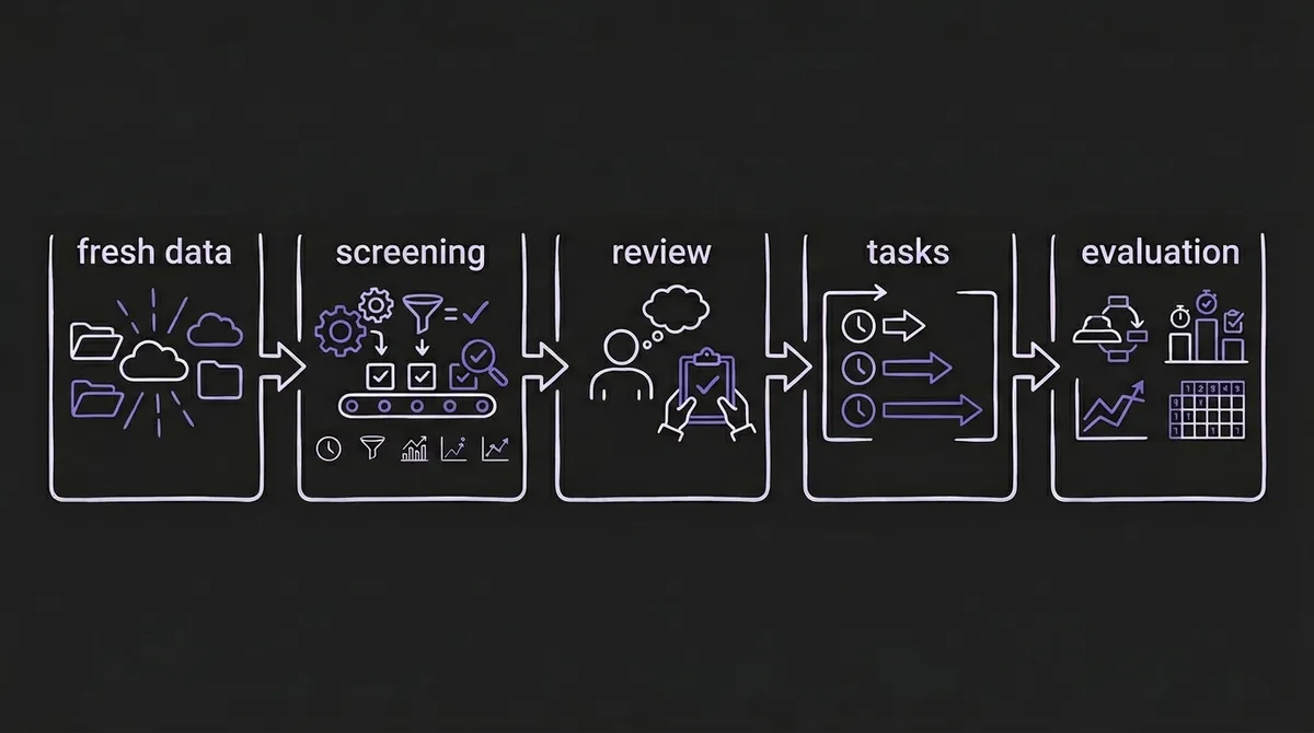
TIME's 50 datasets come from four distinct source categories: official government statistical portals, industrial and academic collaborations, open-access websites, and forecasting competitions. The authors explicitly prioritize novelty — datasets that have never or rarely appeared in existing TSF benchmarks — to minimize the risk of pretraining contamination.

Collecting fresh data is necessary but not sufficient. The paper introduces a rigorous quality assurance pipeline that proceeds in two stages.

#Automated Screening (Five Steps)

Each candidate dataset passes through a five-step automated screening pipeline before any human review:

Step 1 — Timestamp Rectification. Missing or misaligned timestamps are identified and corrected by calibrating to the nearest standard timestamp given the data frequency. This prevents the silent errors that occur when evaluation windows do not align with the series' true temporal structure.

Step 2 — Rule-Based Validation. Variates are automatically flagged for missing rate violations, insufficient length, or negligible temporal dynamics (near-constant series). This catches the uninformative variates that inflate dataset counts in many archives without contributing to evaluation signal.

Step 3 — Statistical Testing. The Ljung-Box test is applied to detect white-noise variates — series with no forecastable temporal structure. Flagged variates are marked for removal. This is a critical step that many benchmarks skip: a variate that is genuinely white noise inflates error scores for all models and adds noise to rankings without testing any meaningful capability.

Step 4 — Extreme Outlier Removal. A local IQR filter with k=9 detects and removes extreme erroneous values while preserving genuine spikes that are part of the domain phenomenon. Detected errors are replaced with the preceding valid observation. The threshold is deliberately conservative: the goal is to remove data artifacts, not to smooth away domain-relevant volatility.

Step 5 — Correlation Check. Pairwise correlations across all variates within each dataset are computed. Highly collinear pairs are flagged for expert review. A high correlation between car park availability readings suggests redundancy; a high correlation between macroeconomic indicators reflects genuine structural dependency. Only expert review can distinguish the two.

All diagnostic results are aggregated into a dataset-level Quality Summary, which feeds the human review stage.

#Human-in-the-Loop Decision Making

The Quality Summary drives a structured human review process guided by both domain expertise and LLM-synthesized context. Human reviewers determine whether to exclude specific series at the series level, remove entire variates at the variate level, or accept the dataset as-is. The review also produces the critical methodological contribution: context-aligned task formulation.

Rather than applying frequency-proportional horizons or one-size-fits-all forecast lengths, the authors define three horizons (Short, Medium, Long) for high-frequency datasets and restrict low-frequency or operationally constrained datasets to a single viable horizon. The forecast length is calibrated to cover practical cycles — full seasonal periods, operational planning windows — ensuring that what the benchmark asks models to do is what practitioners actually need to do.

This context-aware task design is what turns a dataset collection into a benchmark with real operational meaning. It is also what makes TIME's 98 tasks non-redundant even when they span only 50 datasets.

#The 7-Feature Binary Pattern Encoding

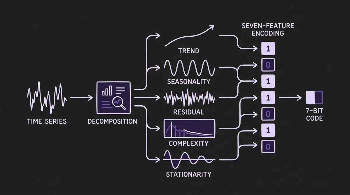
The most technically novel aspect of TIME is its pattern-level evaluation framework. Instead of aggregating model results by dataset or domain label, it aggregates by intrinsic temporal structure — the statistical pattern of each variate, regardless of where it came from.

The framework uses seven structural features derived from STL decomposition and spectral analysis:

F1 — Trend Strength: The proportion of variate variance explained by the trend component. High F1 means the series has a dominant long-range directional movement.

F2 — Trend Linearity: How closely the trend evolves linearly over time. High F2 indicates a trend that progresses at a consistent rate; low F2 indicates curvature, inflection points, or structural breaks in the trend.

F3 — Seasonality Strength: The proportion of variance explained by the seasonal component. High F3 indicates a series dominated by recurring periodic structure.

F4 — Seasonality Correlation: The correlation between consecutive seasonal cycles. High F4 means seasonality is stable and consistent over time; low F4 means the seasonal pattern shifts or evolves.

F5 — Residual ACF-1: The first-order autocorrelation of the STL remainder term. High F5 indicates that significant temporal structure persists after trend and seasonality are removed — the remainder is not white noise.

F6 — Complexity (Spectral Entropy): The normalized spectral entropy of the raw variate. Low F6 (low entropy) means the series has concentrated spectral energy in a few frequencies — it is relatively predictable. High F6 means the spectrum is broadly distributed — it is harder to forecast.

F7 — Stationarity: A binary indicator from the Augmented Dickey-Fuller test. F7=1 indicates a stationary variate (p<0.05); F7=0 indicates non-stationarity.

To convert these continuous features into a usable encoding, each variate is binarized against the population median across all benchmark variates. If a variate's feature value exceeds the population median, it receives a 1 for that feature; otherwise, 0. The result is a 7-bit binary pattern code that can be used to retrieve subsets of variates sharing the same temporal characteristics across different datasets and domains.

This is a more expressive pattern space than QuitoBench's 3-dimensional TSF regime taxonomy (trend strength, seasonality strength, forecastability), which generates 8 cells. TIME's 7-bit encoding supports up to 128 distinct pattern cells, enabling more granular cross-dataset comparisons — at the cost of requiring enough variates per cell for reliable aggregation.

#The 12 Models Evaluated

TIME evaluates a representative cross-section of the TSFM field as of late 2025 and early 2026:

Model	Release	Architecture	Parameters	Multivariate
TimesFM 2.5	Oct 2025	Decoder-only	200M	✗
Chronos-2	Oct 2025	Encoder-only	120M	✓
Kairos	Sep 2025	Encoder-Decoder	23M	✗
Moirai 2.0	Aug 2025	Decoder-only	11M	✗
VisionTS++	Aug 2025	MAE	460M	✓
TiRex	May 2025	xLSTM	35M	✗
Toto	May 2025	Decoder-only	151M	✓
Sundial	May 2025	Decoder-only	128M	✗
TimesFM 2.0	Dec 2024	Decoder-only	500M	✗
Chronos-Bolt	Nov 2024	Encoder-Decoder	205M	✗
Moirai 1.1	Jun 2024	Encoder-only	91M	✓
TimesFM 1.0	May 2024	Decoder-only	200M	✗

The three successive TimesFM versions, two Moirai versions, and two Chronos versions are particularly valuable: TIME's fresh data allows a clean test of whether newer model generations represent genuine capability improvements or benchmark overfitting.

#Overall Results: Top-3 and the Generational Progression

The global leaderboard aggregates task-level normalized metrics (MASE and CRPS relative to Seasonal Naive) using the geometric mean across all 98 tasks. Three models emerge as the consistent leaders: Chronos-2, TimesFM-2.5, and TiRex, occupying the top three positions on both MASE and CRPS.

A structural pattern appears across model generations: newer releases consistently outperform their predecessors.

• TimesFM 2.5 outperforms TimesFM 2.0, which outperforms TimesFM 1.0
• Moirai 2.0 outperforms Moirai 1.1
• Chronos-2 outperforms Chronos-Bolt

On a benchmark with fresh, contamination-free data, this result matters. It means the performance progression seen in model papers is not an artifact of training on the benchmark's test data — newer models are genuinely better. This is not trivial to verify on legacy benchmarks, where contamination risk grows with every passing month.

Among the top five performers, two architectural design trends stand out: decoder-only frameworks (TimesFM 2.5, Toto, Moirai 2.0) dominate the leaderboard, and quantile-based output mechanisms are more common than distributional output among the highest-ranked models. The encoder-decoder architecture tradeoff discussed elsewhere on this site is visible here: for general-purpose zero-shot forecasting, decoder-only architectures are currently holding the performance lead.

#Pattern-Specific Results: Where Rankings Shift

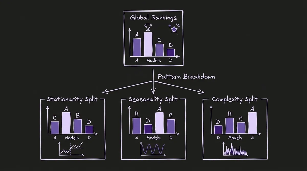
The most actionable output of TIME is the pattern-level analysis, which reveals how model rankings change across different temporal characteristics. Several findings stand out:

#Seasonality Strength: The Great Differentiator

On variates with weak seasonality, model performance differences compress significantly. Most TSFMs cluster around a normalized MASE of approximately 0.7 relative to Seasonal Naive. Even the best models provide only a modest improvement over each other on these series.

On variates with strong seasonality (F3=1), the dispersion widens sharply. The performance gap between stronger and weaker models increases substantially. The implication: seasonality strength is the primary driver of inter-model differentiation in this benchmark. A practitioner whose series are predominantly low-seasonality can expect smaller practical differences between model choices. A practitioner with strongly seasonal series is in the regime where model selection matters most.

This complements the seasonality-based model selection guidance from QuitoBench, which found that DL models outperform foundation models in low-seasonality cells while foundation models win in high-seasonality cells. TIME's pattern analysis reinforces that seasonality is a key discriminating axis.

#Stationarity: The Ranking Flip

The stationarity feature (F7) produces the most dramatic ranking shift in the benchmark. Toto ranks third overall on non-stationary variates but falls to sixth on stationary ones. Conversely, Chronos-2 is the top performer on stationary variates but is surpassed by TimesFM-2.5 on non-stationary data.

This is not a marginal difference — it suggests that Toto and Chronos-2 have meaningfully different inductive biases. Toto was designed for observability metrics, which tend to be non-stationary: they drift with infrastructure load, shift at deployments, and change regime with capacity events. That specialization appears to carry over into TIME's non-stationary slice while limiting performance on stationary series.

Chronos-2's advantage on stationary variates is consistent with its encoder-only architecture and its training objective, which may be better calibrated to series with stable statistical properties.

The practical implication: if you are deploying a TSFM on infrastructure metrics or any domain characterized by non-stationary series (concept drift, regime shifts, ongoing trend), Toto's edge on this slice is worth weighting in your evaluation. If your series are predominantly mean-reverting and stationary, Chronos-2's advantage becomes more relevant.

#Complexity as a Performance Equalizer

High spectral entropy (F6=1, high complexity) acts as a performance equalizer: when variates are spectrally complex, the gap between models compresses. In the high-complexity regime, all models converge toward similar — and generally weaker — relative performance, with the inter-model variance reduced.

In the low-complexity regime (F6=0, concentrated spectral energy), the opposite occurs: better models pull ahead more clearly. The most advanced TSFMs — Chronos-2, TimesFM-2.5 — distinguish themselves most sharply on these structured, lower-entropy series.

This aligns with the intuition that high spectral entropy series present a fundamental forecasting challenge that architectural advantages cannot fully overcome. The ceiling is epistemic: if the series does not have a predictable structure, no model can extract one. The floor is model skill: on series that do have predictable structure, better architectures and pretraining pay off.

#Aggregation Level Instability

TIME's Section 6.3 contains a finding that deserves particular attention from benchmark consumers: rankings computed at task-level aggregation and variate-level aggregation do not agree. The paper finds that while feature-specific pattern rankings are generally consistent with the overall task-level rankings at the top (Chronos-2 and TimesFM-2.5 remain leaders), the middle of the leaderboard shifts depending on whether results are aggregated at the task or variate level.

This is a methodological insight with broad implications. Every benchmark makes an implicit choice about aggregation level, and that choice affects which model appears to win. Task-level aggregation (the standard practice) weights datasets equally regardless of how many variates they contain. Variate-level aggregation weights individual prediction targets equally regardless of which dataset they come from. Neither is universally correct — the right choice depends on what you are measuring and how you plan to deploy the model.

TIME's architecture supports both views through its interactive leaderboard, enabling practitioners to choose the aggregation that matches their deployment context.

#The Visualization Argument

The paper makes a point about quantitative metrics that is easy to dismiss and should not be. In one motivating example, a TimesFM 2.5 forecast achieves MASE=0.662 and MAE=1.12 on a test window — metrics that appear favorable — but the visualization reveals that the forecast completely fails to capture a distinct spike structure in the series. The model has produced a conservative, near-flat forecast that happens to achieve acceptable error scores by matching the local mean.

This "safe mediocrity" failure mode — where a model produces low-variance predictions that score well numerically but miss the structural content of the series — is real and practically consequential. A forecast that smooths over genuine spikes provides false confidence in planning scenarios that depend on capturing extremes. The paper argues that quantitative rankings need to be supplemented with qualitative visualization, and TIME's interactive leaderboard integrates both.

The relevant implication for practitioners: when comparing models, requesting that they forecast a set of challenging series from your domain and visually inspecting the predictions is not optional. A model that produces flat forecasts on spiky series is not useful even when its aggregate MASE looks competitive.

#Practical Takeaways

TIME's combined findings yield several actionable guidelines for TSFM practitioners:

Verify stationarity before selecting a model. Run an Augmented Dickey-Fuller test on a sample of your training data. If most series are non-stationary, Toto's architecture bias becomes a meaningful edge. If most are stationary, Chronos-2's performance advantage is more likely to hold.

Assess seasonality strength to predict how much model choice will matter. If your series have weak or absent seasonality, the performance gap between top-tier models will be small in this benchmark. If your series are strongly seasonal, the choice of model family is likely to produce materially different outcomes.

Use context-aligned horizon evaluation. Do not evaluate models on arbitrary horizon lengths. The horizon that matters is the one your operational process actually uses. TIME's task-centric approach formalizes this; your internal evaluation should do the same.

Treat aggregate leaderboard rankings as directional, not definitive. The finding that rankings shift by aggregation level is a caution against relying on a single aggregate score. Pattern-level benchmarks like TIME give you a more granular starting point, but you still need to evaluate on data representative of your domain and statistical regime.

Watch for the conservative-prediction failure mode. Models that produce good aggregate scores by generating near-constant forecasts may score worse on metrics that directly penalize structural misses. Inspect predictions qualitatively, especially on series with known spike or regime-change behavior.

Trust the generational progression — with fresh data. On TIME's contamination-free evaluation, newer model generations are genuinely better. This is a stronger signal than leaderboard improvements on legacy benchmarks, where contamination confounds interpretation. For model selection decisions, this means prioritizing recent releases when they have been evaluated on fresh data.

#How TIME Fits into the Benchmarking Landscape

TIME, QuitoBench, GIFT-Eval, FEV Bench, BOOM, and Impermanent each address a distinct facet of the TSFM evaluation problem:

• GIFT-Eval provides broad multi-domain coverage with contamination-aware dataset selection
• FEV Bench tests pure zero-shot skill across 29 datasets with explicit contamination tracking
• BOOM provides domain-specific evaluation on real production observability metrics
• Impermanent tests temporal generalization under ongoing distribution shift
• QuitoBench uses a 3-dimensional regime taxonomy to expose context-length crossovers and forecastability effects
• TIME introduces operational task alignment and a 7-feature variate-level pattern encoding that enables cross-dataset structural comparisons

No single benchmark captures everything. TIME's distinctive contribution is the human-in-the-loop construction pipeline that produces genuinely fresh, integrity-verified data with operationally meaningful task definitions — combined with a pattern encoding system that enables granular insights into when and why specific models succeed.

For practitioners who have been using aggregate benchmark scores to make model selection decisions, TIME's core message is that the aggregation level matters, the temporal patterns of your specific data matter, and visual verification of model behavior is not optional. The benchmark provides the infrastructure to act on all three insights at once.

---

Primary sources: TIME paper (arXiv:2602.12147), TIME interactive leaderboard on HuggingFace, TIME dataset on HuggingFace, TIME source code on GitHub.