IBM FlowState: The First Sampling-Rate-Invariant Time Series Foundation Model

Most time series foundation models make the same architectural bet: tokenize your series into patches, feed them through a transformer, and produce a fixed-length forecast from a linear or MLP head. IBM Research's FlowState breaks with all three steps. It drops the transformer entirely in favor of a State Space Model encoder, uses no patching, and replaces the fixed output head with a Functional Basis Decoder that produces a continuous forecast function rather than a fixed-length vector. The result is a model that not only matches models ten times its size on GIFT-Eval but can also adjust to an entirely different sampling rate at inference time — without any retraining.

This post is a technical deep dive into FlowState's architecture, training scheme, and practical deployment considerations. It covers the material that the brief mention in our 2026 TSFM toolkit guide does not.

The Problem FlowState Solves

Existing TSFMs have three connected limitations that stem from the same root cause: their architectures are designed for discrete, fixed-rate, fixed-length inputs and outputs.

Sampling rate rigidity. A model pretrained on hourly data implicitly learns the temporal dynamics at that frequency. Applying it to 15-minute or daily data requires either resampling the series to match the training frequency (losing information) or retraining from scratch on multi-frequency data (expensive). Most models that support multiple frequencies solve this by including all frequencies in pretraining — they memorize patterns at each scale rather than adapting dynamically.

Fixed forecast horizons. Most TSFMs commit to a specific output length at architecture design time. Their output heads (linear layers or small MLPs) have a fixed number of output neurons corresponding to the number of forecast steps. Changing the horizon requires retraining or awkward inference tricks.

Context length inflexibility. Patching-based models process a fixed number of patches per forward pass. When the available context is shorter or longer than training context, performance degrades — the model sees a differently-sized input than it was optimized for.

FlowState addresses all three by moving computation into a timescale-invariant coefficient space rather than the raw time-step space.

Architecture: SSM Encoder + Functional Basis Decoder

FlowState is an encoder-decoder architecture, but both components are atypical by current TSFM standards.

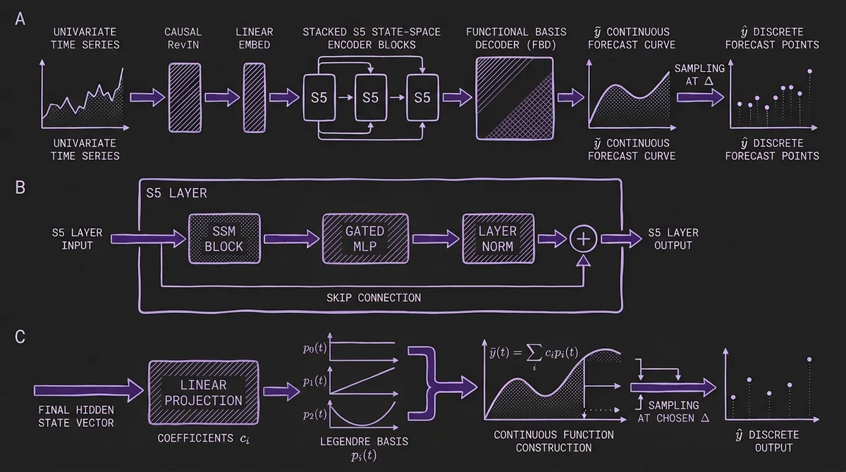
SSM Encoder (S5 Layers)

The encoder is built from a stack of S5 layers — the Simplified State Space Sequence model variant. Unlike transformers, which compute pairwise attention scores between all positions, an SSM updates a hidden state sequentially:

s_t = Ā · s_{t-1} + B̄ · x_t
h_t = C̄ · s_t + D̄ · x_t

The matrices (Ā, B̄, C̄, D̄) are derived from learned continuous parameters (A, B, C, D) discretized with a time-step parameter Δ. Critically, this discretization is the key to sampling rate adaptation: by scaling Δ at inference time, the SSM can produce nearly identical internal representations regardless of the input frequency. A model pretrained on daily data can generalize to monthly or hourly data through this mechanism.

Each S5 layer adds an MLP on top of the SSM block, with skip connections that allow raw inputs to propagate to later encoder layers. FlowState stacks several such layers to build a deep SSM encoder.

One practical difference from most TSFMs: FlowState processes the time series as-is, without patching. While PatchTST, Chronos-Bolt, TimesFM, and most other modern TSFMs group consecutive time steps into patches before feeding them to the model, FlowState feeds individual time steps directly to the SSM. The sequential structure of the SSM already provides efficient handling of long sequences through its linear recurrence.

Functional Basis Decoder (FBD)

The output of the SSM encoder's final layer is a vector of activations at the last time step. Most architectures would feed this directly into a linear layer to produce a fixed-length forecast. FlowState interprets these activations as coefficients of a continuous function instead.

Specifically, the FBD interprets the encoder output as coefficients c_i of a polynomial basis (Legendre polynomials by default, for consistency with the HiPPO initialization used in the SSM). From these coefficients, it constructs a continuous forecast function:

ỹ = Σ_i c_i · p_i(a, b)
ŷ = sample(ỹ, Δ)

where p_i(a, b) is the i-th basis function evaluated over a normalized interval, and the continuous function ỹ is then sampled at equally spaced intervals with spacing Δ to produce the discrete forecast.

This has three practical consequences:

1. Variable-length forecasts without retraining. Because the output is a sampled continuous function, you can request any forecast horizon at inference time without changing any weights.
2. Sampling rate adaptation. The same Δ scaling parameter that adapts the SSM encoder also controls the sampling of the FBD output. Change Δ and both the encoder's temporal dynamics and the output sampling rate shift in tandem.
3. Principled continuous-time representation. The FBD draws from the same mathematical lineage as the HiPPO initialization, so the coefficient-space representation has a well-understood relationship to the underlying signal.

Causal Normalization

A subtle but important implementation detail: FlowState uses a causal variant of RevIN rather than standard RevIN. Standard RevIN normalizes each time series using the mean and standard deviation of the entire context window. This creates a problem for FlowState's parallel prediction training scheme (described next) — if normalization uses future values, the model can learn to exploit that information leak.

FlowState instead normalizes each time step using a running mean and running standard deviation up to that step:

μ_{r,t} = cumsum(x_{1:t}) / t
σ²_{r,t} = cumsum((μ_{r,t} - x_{1:t})²) / t
x̃_t = (x_t - μ_{r,t}) / σ_{r,t}

Forecasts are then de-normalized using the statistics at the last context time step. This ensures strict causality during both training and inference.

Parallel Prediction Training

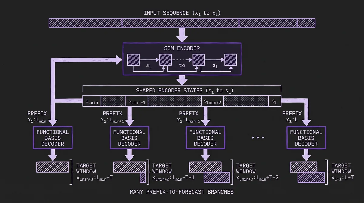
FlowState's training scheme is among its most distinctive contributions. Standard TSFM training generates one forecast per context-target pair in the training data. FlowState can generate forecasts from every context prefix between L_min and L in parallel.

The scheme exploits the SSM's inherent parallelizability. Because the SSM processes input causally (each step depends on previous steps), the encoder can process a long context sequence in a single parallel pass and expose all intermediate states simultaneously. FlowState then makes predictions from every context length from L_min to L, with each prediction having its own target window:

• Forecast from context x_{1:L_min} targets x_{L_min+1:L_min+T}
• Forecast from context x_{1:L_min+1} targets x_{L_min+2:L_min+T+1}
• ...
• Forecast from context x_{1:L} targets x_{L+1:L+T}

For L = 2048 and L_min = 20, this produces 2,029 training examples from a single sequence. The benefits are compound: training data utilization improves dramatically, and the model becomes inherently robust to context lengths it has not seen at training time since it is explicitly trained on every prefix length.

Benchmark Results

FlowState was evaluated on two benchmarks under zero-shot conditions: GIFT-ZS (the contamination-aware subset of GIFT-Eval excluding the 18 tasks present in the Chronos pretraining corpus) and Chronos-ZS (the FEV Bench zero-shot evaluation suite).

GIFT-ZS

On the 79-task GIFT-ZS subset, FlowState(G) — trained on the GIFT-Eval pretraining split — sets new state-of-the-art performance on both MASE and CRPS, outperforming all baseline models including TiRex (which holds the top spot on the full GIFT-Eval leaderboard when data overlap is not controlled for). This is despite FlowState having fewer than 10M parameters while the next best models are an order of magnitude larger.

The IBM documentation notes that FlowState held the #1 position on the GIFT-Eval leaderboard as of September 9, 2025, and #3 as of October 2, 2025 — reflecting continued competition as other teams update their submissions to the live leaderboard.

Chronos-ZS

FlowState(T) — trained on the TiRex pretraining corpus (which avoids overlap with Chronos-ZS evaluation data) — achieves competitive WQL and MASE on the Chronos zero-shot benchmark suite, comparable to or better than models in its size class.

The Efficiency Angle

The headline figure in the FlowState model card is the parameter efficiency: FlowState is more than 10x smaller than the three next-best models on the GIFT-Eval leaderboard, yet outperforms all of them on GIFT-ZS. This is a stronger claim than what IBM established for Granite TTM, which matched models 40x its size but did not lead the leaderboard outright.

Practical Deployment

Sampling Rate Adaptation in Practice

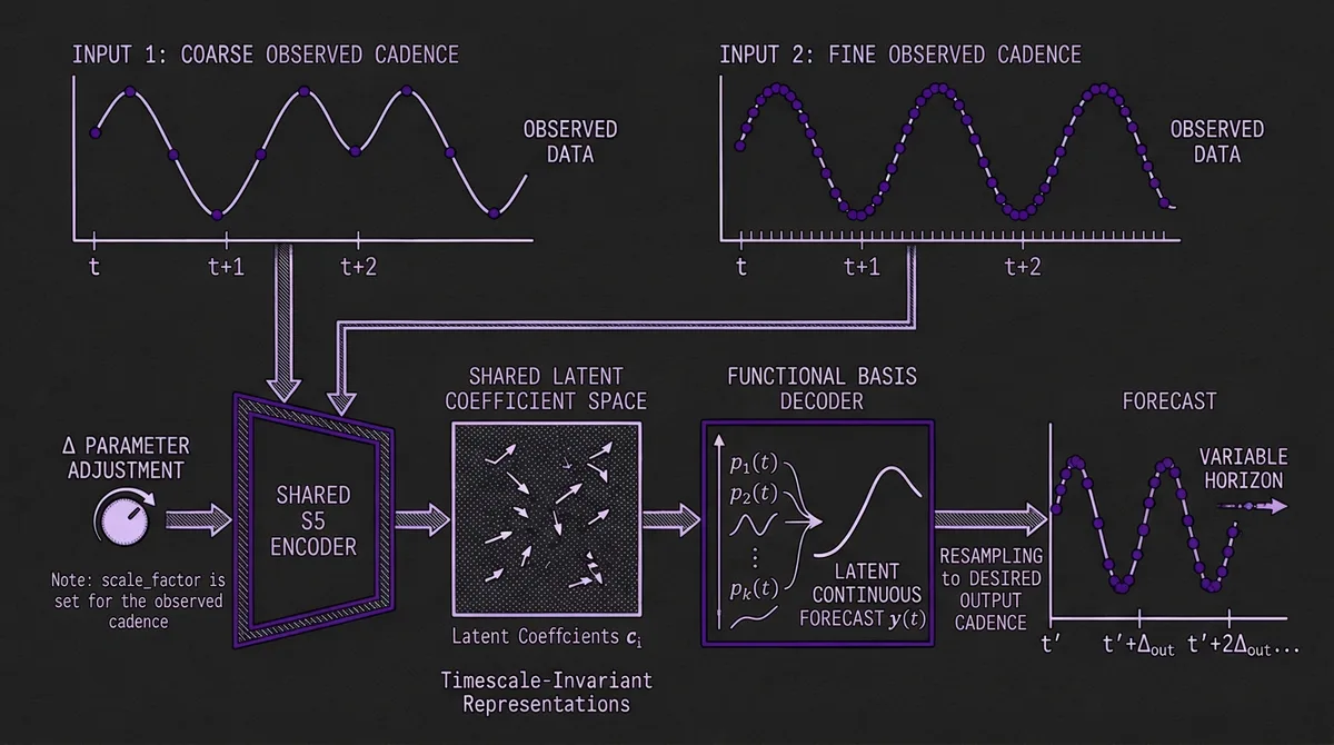
The scale_factor (sΔ) parameter is the key dial for adapting FlowState to your data's temporal scale. The recommended values from the model card:

Sampling Rate	Recommended scale_factor
15-minute	0.25
30-minute	0.5
Hourly	1.0
Daily (weekly cycle)	3.43
Daily (no weekly cycle)	0.0656
Weekly	0.46
Monthly	2

The underlying formula is scale_factor = 24 / seasonality, where 24 is the base seasonality used during pretraining and seasonality is the number of time steps per repeating cycle in your data. For 15-minute data with a 24-hour daily cycle, one cycle contains 96 steps (4 per hour × 24 hours), giving scale_factor = 24 / 96 = 0.25. For daily data with a weekly cycle, one cycle contains 7 steps, giving scale_factor = 24 / 7 ≈ 3.43. If the seasonality is unclear, IBM recommends experimenting with different values and selecting based on held-out accuracy.

One practical constraint: the model card recommends forecasting no more than 30 seasons into the future. Beyond that, the continuous-function approximation degrades. For data with a 96-step daily cycle, this means a maximum horizon of 2,880 steps — more than adequate for most production use cases.

Probabilistic Forecasts

FlowState produces probabilistic forecasts out of the box, outputting quantile estimates at multiple levels. This distinguishes it from TimesFM (which produces point forecasts by default) and aligns it with Chronos and Moirai for applications requiring calibrated prediction intervals.

Inference and Current Public Implementation

The public FlowState checkpoint is available through the Hugging Face model hub and the IBM granite-tsfm library. The released granite-tsfm implementation currently exposes FlowState as a zero-shot forecasting model, and its current FlowStateModel path raises an error when past_values contains more than one channel, so practitioners should treat the public release as univariate in its current form:

from tsfm_public import FlowStateForPrediction
import torch

predictor = FlowStateForPrediction.from_pretrained(
    "ibm-granite/granite-timeseries-flowstate-r1"
).to("cuda")

# context shape: (context_len, batch_size, n_channels)
time_series = torch.randn((2048, 32, 1), device="cuda")

forecast = predictor(
    time_series,
    scale_factor=0.25,       # 15-minute data with daily cycle
    prediction_length=960,   # 10 days ahead at 15-min resolution
    batch_first=False,
)
print(forecast.prediction_outputs.shape)  # torch.Size([32, 960, 1])
print(forecast.quantile_outputs.shape)    # torch.Size([32, 9, 960, 1])

How FlowState Fits in the TSFM Landscape

The TSFM field is now characterized by three architectural families: encoder-only (Chronos-Bolt, MOMENT, Moirai), decoder-only (TimesFM, Toto, Lag-Llama), and encoder-decoder (original Chronos, TFT). FlowState adds a fourth: SSM-based continuous-time models.

Each family has a different cost-benefit profile for common production workloads:

	FlowState	Encoder-Only	Decoder-Only
Parameter count	~9M (smallest)	14M–711M	200M–8.3B
Inference style	Single pass (SSM recurrence)	Single pass	Autoregressive
Horizon flexibility	Continuous (any length)	Fixed per head	Flexible
Sampling rate adaptation	Native (via Δ scaling)	None (needs resampling)	None
Probabilistic output	Yes (quantiles)	Model-dependent	Via sampling
Published zero-shot result	GIFT-ZS SOTA in paper	Strong	Strong

The most practically significant differentiator is sampling rate adaptation. If your forecasting problem involves multiple data sources at different frequencies — a common scenario in supply chain, energy, or IoT settings — FlowState eliminates a category of preprocessing complexity that other TSFMs require you to handle externally.

The Novelty of SSMs for Time Series

State Space Models have been a strong presence in sequence modeling since Gu et al. introduced S4 in 2021, and subsequent variants (S5, Mamba, Mamba2) have refined the architecture considerably. Their appeal for time series is theoretical: SSMs are mathematically continuous-time systems, making them a natural fit for temporal data. The HiPPO initialization — which FlowState adopts — was specifically designed to give SSM hidden states a polynomial-basis interpretation of the input history, which is exactly what the FBD exploits.

The challenge has been that SSMs in the NLP domain have struggled to match transformer quality on some tasks. For time series, where the data is continuous-valued, lower-dimensional, and has strong temporal regularity, SSMs have significant structural advantages that the FlowState paper quantifies on GIFT-Eval.

This is worth monitoring. If SSM-based TSFMs continue to outperform transformers at smaller parameter counts — as the FlowState results suggest — the architectural diversity of the TSFM space will expand beyond the encoder/decoder/encoder-decoder taxonomy that currently dominates. For benchmarking practitioners, this means tracking a fourth model family with qualitatively different failure modes and strengths.

When to Choose FlowState

FlowState is the right choice when one or more of the following is true:

Multi-frequency pipelines. If you operate on data collected at multiple sampling rates (sensor networks, multi-source IoT, blended financial data), FlowState's native Δ-scaling eliminates the need to maintain separate models per frequency or to resample and lose resolution.

Parameter-efficient zero-shot forecasting. At under 10M parameters, FlowState is comparable to Granite TTM in size while posting stronger published GIFT-ZS results than larger baseline models in the paper and model card.

Variable-horizon forecasting from a single model. If your application needs to serve multiple horizon lengths (a common API pattern), FlowState's continuous FBD outputs any horizon without retraining or multiple model variants — within the recommended 30-season limit for reliable forecast quality.

Strong out-of-the-box zero-shot performance. If your priority is maximizing zero-shot accuracy before committing to fine-tuning infrastructure, FlowState offers one of the strongest published starting points in its size class.

Where FlowState is less suited: workloads that depend on multivariate cross-channel modeling in the current public granite-tsfm release, or scenarios where you need fine-tuning workflows and ecosystem depth beyond the current zero-shot public checkpoint.

FlowState is available on TSFM.ai alongside Granite TTM, Chronos-Bolt, TimesFM, and Moirai — letting you benchmark it against any alternative on your own data through a single API without managing model infrastructure.